Lesson 13 official topic

[ganesh.bhat]

I was just going through the 03_backprop.ipynb and came across a question. The loss is measured using ‘res’ in the below code. Should it be diff.pow(2).mean() (MSE) since this is on the training set (x_train) and not x_valid?

‘res’ refers to running the model on x_valid.

res = model(x_valid)

Please correct my understanding if it is not correct.

def forward_and_backward(inp, targ):
# forward pass:
l1 = lin(inp, w1, b1)
l2 = relu(l1)
out = lin(l2, w2, b2)
diff = out[:,0]-targ
loss = res.pow(2).mean()

# backward pass:
out.g = 2.*diff[:,None] / inp.shape[0]
lin_grad(l2, out, w2, b2)
l1.g = (l1>0).float() * l2.g
lin_grad(inp, l1, w1, b1)

We call the function using x_train and y_train.

forward_and_backward(x_train, y_train)

[DeedaxInc (Dahir)]

There’s this thing about backprop that, once it clicks for you (you understand it), you immediately want to share because you know how exhausting it can be.

I made a video trying to explain backprop math as well. Of course the one from Jeremy and Andrej are miles better, but maybe check out this one too coming from a student like you.

Part 4: Backward Propagation

I am so open to corrections and suggestions.

[devforfu (Ilia)]

By the way, I am still unsure why pytorch computes bias differently from what I did. I think it could be some minor detail about vector arithmetic. But still, it would be good to clarify that. I have a notebook where I compare my custom implementation with what PyTorch is doing.

---

Here is a snippet I created:

W1 = grad(torch.eye(4))
b1 = grad(torch.ones(X.shape[0], W1.shape[-1]))
W2 = grad(t([1., 0., -1., 1.]).unsqueeze(-1))
b2 = grad(torch.ones((X.shape[0], W2.shape[1])))

(F.relu(F.relu(X@W1 + b1)@W2 + b2) - y).pow(2).mean().backward()

mse = MSE()
lin1, rel1 = Linear(W1, b1), ReLU()
lin2, rel2 = Linear(W2, b2), ReLU()

mse(rel2(lin2(rel1(lin1(X)))), y)
mse.backward()
rel2.backward()
lin2.backward()
rel1.backward()
lin1.backward()

[test(x.g, x.grad) for x in (W1, W2, b1, b2)];

It tests if two implementations produce the same result. It works for W1 and W2, but for biases, I get different results:

b1.g, b1.grad

(tensor([ 2.,  0., -2.,  2.], grad_fn=<SumBackward1>),
 tensor([[ 0.,  0., -0.,  0.],
         [ 2.,  0., -2.,  2.],
         [ 0.,  0., -0.,  0.]]))

And, in this case, at least, it is clear that b1.g == b1.grad.sum(0). (That’s what I do in the implementation.)

class Linear(Module):
    def __init__(self, W, b):
        super().__init__()
        self.W, self.b = W, b
    def forward(self, inp): return inp @ self.W + self.b
    def backward(self):
        i, o = self.inp, self.out
        i.g = o.g @ self.W.t()
        self.W.g = i.t() @ o.g
        self.b.g = o.g.sum(0)  # same bias for all rows
    def __repr__(self):
        return f"{self.__class__.__name__}({list(self.W.shape)})"

Do you know what’s going on there?

Also, I trained a trivial model that predicts the number five using MLP plus cross-entropy loss and got 65-70 percent of accuracy. So, the implementation is not completely off. However, it doesn’t mean it works exactly as it should either.

---

@krasin Yes, that’s a good point! I think now I understand why it works like this. It also reminded me of a picture from some textbook about perceptron, with a neuron plus bias, like this one.

And here it is clear that one just adds the same scalar to each layer, so, it is a vector, and not a matrix. I mean, I saw it many times and even coded it via representing bias as an additional constant column added to the data… Anyway, there are so many ways to get things wrong in the ML

[krasin]

Nice notebook @devforfu! Your implementation is correct, just the bias should be vector, not matrix (as discussed in the previous post). Try with:

    W1 = grad(torch.eye(4))
    b1 = grad(torch.ones(W1.shape[-1]))
    W2 = grad(t([1., 0., -1., 1.]).unsqueeze(-1))
    b2 = grad(torch.ones((W2.shape[1])))

Another option is

    W1 = grad(torch.eye(4))
    b1 = grad(torch.ones(1, W1.shape[-1]))
    W2 = grad(t([1., 0., -1., 1.]).unsqueeze(-1))
    b2 = grad(torch.ones((1, W2.shape[1])))

[Najdorf (Ramamurthi)]

Hi ,

Can someone help me out here to point out what’s wrong with this ?

This is a close replica of the script to create backprop from scratch .

import torch
X = torch.randn(5000 , 764)
y = torch.randint(0, 9, (5000,))

import torch.nn.functional as F

# class Module():
#     def forward(self,*args):
#         raise NotImplementedError("Forward Method not implemented")
#     def __call__(self,*args):
#         self.args = args
#         self.out = self.forward(*args)
#         return self.out
#     def backward(self): self.bwd(self.out, *self.args)
#     def bwd(self,*args): raise Exception('not implemented') 

    
class Module():
    def __call__(self, *args):
        # import pdb ; pdb.set_trace()
        self.args = args
        self.out = self.forward(*args)
        return self.out

    def forward(self): raise Exception('not implemented')
    def backward(self): self.bwd(self.out, *self.args)
    def bwd(self): raise Exception('not implemented')
    
    
class Linear(Module):
    def __init__(self, ni , no):
        super().__init__()
        self.w = torch.randn(ni, no).requires_grad_()
        self.b = torch.zeros(no).requires_grad_()
    def forward(self,x):
        return x@self.w + self.b
    def bwd(self , out , inp):
        inp.g = self.out.g @ self.w.t()
        self.w.g = inp.t() @ self.out.g
        self.b.g = self.out.g.sum(0)


class Relu(Module):
    def __init__(self):
        pass
    
    def forward(self,x):
        self.out = x.clamp_min(0.)
        return self.out
    
    def bwd(self,out,inp):
        inp.g = (inp>0).float() * out.g
        


class Mse(Module):
    def forward (self, inp, targ): return (inp.squeeze() - targ).pow(2).mean()
    def bwd(self, out, inp, targ): inp.g = 2*(inp.squeeze()-targ).unsqueeze(-1) / targ.shape[0]
                
        
        

class Model(Module):
    def __init__(self , num_hidden_layers , ni  , nh , no):
        
        
        self.relu = Relu()
        
        # Stacking layers
        self.l1 = [ Linear(ni,nh) , self.relu ]
        self.hidden_layers = []
        for _ in range(num_hidden_layers-1):
            self.hidden_layers.append(Linear(nh,nh))
            self.hidden_layers.append(self.relu)
        self.out_layer = [Linear(nh,no)]
        
        self.layers = self.l1 + self.hidden_layers + self.out_layer
        self.mse = Mse() 
        
        
    def forward(self,x):    
        
        for layer in self.layers:
            # import pdb ; pdb.set_trace()
            x = layer(x)
        return x
    
    def __call__(self,x, y):
        x = self.forward(x)
        self.loss = self.mse(x , y)
        return self.loss
    
    def backward(self,*args):
        self.loss.backward()
        for l in reversed(self.layers):
            l.backward()
    
            
                                     
    
ni = X.shape[1]
nh = 32
no = 1
num_hidden_layers = 1
model = Model(num_hidden_layers,ni,nh,no)
loss = model(X,y)
model.backward()

When i execute this , i get an error saying

---------------------------------------------------------------------------
AttributeError                            Traceback (most recent call last)
Cell In[163], line 107
    105 model = Model(num_hidden_layers,ni,nh,no)
    106 loss = model(X,y)
--> 107 model.backward()

Cell In[163], line 96, in Model.backward(self, *args)
     94 self.loss.backward()
     95 for l in reversed(self.layers):
---> 96     l.backward()

Cell In[163], line 26, in Module.backward(self)
---> 26 def backward(self): self.bwd(self.out, *self.args)

Cell In[163], line 38, in Linear.bwd(self, out, inp)
     37 def bwd(self , out , inp):
---> 38     inp.g = self.out.g @ self.w.t()
     39     self.w.g = inp.t() @ self.out.g
     40     self.b.g = self.out.g.sum(0)

AttributeError: 'Tensor' object has no attribute 'g'
​

[wills]

@Najdorf seems like self.out.g is missing g. This is supposed to be the gradient calculated from the layer in front of the Linear layer, MSE in this case.

Looking at Model class you name the instance of Mse as self.mse instead of self.loss in the notes. Which means that when you call self.loss.backward() in Mse model’s backward method, the gradient was not calculated.

You can change the call the backward in Model to the following and I think it should work

class Model(Module):
   ...
       def backward(self,*args):
        self.mse.backward()
        for l in reversed(self.layers):
            l.backward()

You can also change your variable names to match the notes so it’s easier to compare

[wills]

I got an error when I was trying to run log_softmax using our implementation of logsumexp

def logsumexp(x):
    m = x.max(-1)[0]
    return m + (x-m[:,None]).exp().sum(-1).log()
     

def log_softmax(x): return x - logsumexp(x)

but realized that it was due to invalid broadcasting

def log_softmax(x): return x - logsumexp(x)[:, None]

Hopefully this is useful to someone else as well

[ForBo7 (Salman Naqvi)]

I went through the “The Matrix Calculus You Need for Deep Learning” paper and it was a thoroughly enjoyable read! It felt good being able to intuitively solve all the problems posed in the paper. I also came out with a generally better understanding of derivatives, too.

I highly recommend going through this paper and solving all the problems in it if you want a better understanding of backpropagation: it’s really just a big fat chain rule problem.

After going through this paper, I compiled all the problems posed in the paper into a single PDF for easier practice. You can access the PDF here: https://forbo7.github.io/misc/matrix_calculus_practice.pdf

Do let me know of any corrections or improvements!

[ForBo7 (Salman Naqvi)]

Could someone please help me figure out why my calculated gradients differ from PyTorch.

I have a neural network with 2 layers.

• The first layer is a linear combination/dot product plus a ReLU: l_1 = \text{max}(0, \vec{x} \cdot \vec{w}_1 + b_1)
• The second layer is simply the linear combination/dot product: l_2 = l_1 \cdot \vec{w}_2 + b_2

All in all, it comes out to look like this.

\text{max}(0, \vec{x} \cdot \vec{w}_1 + b_1) \cdot \vec{w}_2 + b_2

My loss function is MSE and hence comes out looking like this, where N is the number of samples, and y_i is the corresponding target.

\frac{1}{N} \sum^N_{i=1} (y_i - (\text{max}(\vec{w}_1 \cdot \vec{x}_i) \cdot w_2 + b_2))^2

After doing a bunch of maths, I think I’m quite sure that the gradients for w_1 is given by the following simplified formula, where l_2 is the output of the second layer.

\frac{\partial \text{MSE}}{\partial \vec{w}_1} = \frac{2}{N} \sum^N_{i=1} (l_2 - y_i) \vec{w}_2^T \vec{x}^T_i

Now I’m having a bit of trouble implementing this backpropagation formula in Python. Below is my implementation.

w1_gs = (2/trn_x.shape[0]) * ((l2 - trn_y[:, None] * w2.T)[:, None, :] * trn_x[..., None]).sum(0)

The problem is that the gradients obtained from this snippet differ from that calculated by PyTorch using the .backward() method, and I don’t know why or what I’m messing.

For context, this is Jeremy’s implementation.

    # forward pass:
    l1 = lin(inp, w1, b1)
    l2 = relu(l1)
    out = lin(l2, w2, b2)
    diff = out[:,0]-targ
    loss = diff.pow(2).mean()
    
    # backward pass:
    out.g = 2.*diff[:,None] / inp.shape[0]
    lin_grad(l2, out, w2, b2)
    l1.g = (l1>0).float() * l2.g
    lin_grad(inp, l1, w1, b1)

def lin_grad(inp, out, w, b):
    # grad of matmul with respect to input
    inp.g = out.g @ w.t()
    w.g = (inp.unsqueeze(-1) * out.g.unsqueeze(1)).sum(0)
    b.g = out.g.sum(0)

You can view my notebook here. The relevant section is “Gradients and backward pass”.

I’d really appreciate any input or help!

[mannypardo]

You’re missing a parenthesis in your code. In you’re code you’re multiplying (l2 - trn_y[:, None] * w2.T)
It should be (l2 - trn_y[:, None] )* w2.T

[ForBo7 (Salman Naqvi)]

I decided to break down my massive formula and implement it bit by bit, and I finally obtained the same gradients as that of PyTorch. It also helped me better understand Jeremy’s implementation, as mine ended up being similar to his.

My step-by-step implementation of the algorithm to obtain the weights of w1/w_1:

diff = (trn_y[:, None] -l2)
loss.g = (2 / trn_x.shape[0]) * diff
diff.g = loss.g * -1
l2.g = diff.g @ w2.T
l1.g = l2.g * (l1 > 0).float()
w1.g = (l1.g[:, None, :] * trn_x[..., None]).sum(0)

Note for next time: don’t implement an algorithm all in one line; break it down and implement it bit by bit.

Turns out that I was multiplying w2.T in the wrong place as @mannypardo pointed out, that I was multiplying w2.T when I should rather be taking the dot product, and that I left out the crucial derivative for the ReLU (\begin{cases} 0 &l_1 ≤ 0 \\ 1 &l_1 > 0 \end{cases} // (l1 > 0).float()
).

[ForBo7 (Salman Naqvi)]

Ah yes, success! Successfully implemented backpropagation myself from scratch for all weights and biases.

w1, b1, w2, b2 contain the gradients calculated with my own backpropagation algorithm, while w1_, b1_, w2_, b2_ contain PyTorch’s gradients.

[Laulito]

Hey guys,

I wanted to share a drawing with you that I’ve created with Inkscape to help me visualise the whole process:

Here I tried to visualise the MLP that we use on the MNIST dataset. In the visualisation I’ve passed a single image with its 28x28 = 784 pixels through the MLP (X @ W = Y) resulting in 10 values for the resulting first line of what would be our output matrix Y like Jeremy explains it around 14:15 in the video 13 of the fast.ai course (practical deep learning for coders part 2).

Now I can feel that I’m really really close to understand the whole concept but there is still missing something important: The deciding factor in this simple linear setup would be the weights - so by backpropagating a loss to update the weights we would eventually end up getting “better weights” so the resulting matrix Y would create a smaller loss if we go in forward direction again.

But what is it we are actually comparing our values of Y with? Lets assume we just multiply our matrix X with random values of a random matrix W we would get a resulting matrix Y that causes a certain loss. But wouldn’t we need to know beforehand how a “perfect” result of Y needs to look like to make an equation out of these two values? For example (Yperfect - Yrandom)^2 = Loss? What gives the MLP the “hint” that it’s W values are either too small or too big? Wouldn’t we need a Yperfect?

I’ve read the maths post from Kaushik Sinha and there he puts the activations inside the loss equation J = 1/N Sum of N (a(i) - y(i))^2, but for that situation we used a ReLU activation function.

Would I need to do the same for a linear model? So the exact same procedure, just with the difference that my activation funtion inside a neuron would be a linear function instead of a ReLU?

If so, maybe someone can help me with my original drawing -
X @ W = Y would give me one part of our loss equation. But A is still missing (Loss J = 1/N Sum of N (a(i) - y(i))^2). How would I calculate a first vector of the matrix A to compare it to the first line (first vector) of the Y matrix in the image that I’ve drawn assuming that we have a linear activation function?

Would we just multiply Y by any linear value? So, for example
A = Y * linear value? How would that be any good?

I hope you don’t get upset with me right now as I’m a bit confused with this lesson, but as soon as I understand this last piece I think that I’ll understand it all. Chain rule, SGD and the whole math behind the lesson is not a problem at all for me. It’s more of an “engineering problem” right now, because I’m not able at all to visualise a simple linear loss function, which is crucial for me to understand it though.

If I can add that last part to my drawing, integrating a visualisation of the loss function as well, I guess it could be a great way to further deepen the understanding of video 13 and essentially of the whole MLP concept in general.

Thanks for your time and for this great course, thanks for all the effort guys, been really educational so far, see forward hearing from you

[ForBo7 (Salman Naqvi)]

But what is it we are actually comparing our values of Y with? Lets assume we just multiply our matrix X with random values of a random matrix W we would get a resulting matrix Y that causes a certain loss. But wouldn’t we need to know beforehand how a “perfect” result of Y needs to look like to make an equation out of these two values? For example (Yperfect - Yrandom)^2 = Loss? What gives the MLP the “hint” that it’s W values are either too small or too big? Wouldn’t we need a Yperfect?

The lower the loss is, the closer the predicted values are to the actual values. That’s what’s guiding the system to the right weights.

Let’s say we have the weight w. The gradient we find for it is 2. This means incrementing w by one would increase the loss by 2. So what we want to do is decrement w by one so the loss decreases by 2.

Similarly, let’s say we have the bias b. The gradient we find for it is -2. This means incrementing b by one would decrease the loss by 2, which is what we want. We don’t want to decrement b, else it would increase the loss by 2.

Remember, derivatives tell us how much a change in one value would change another value.

I’ve read the maths post from Kaushik Sinha and there he puts the activations inside the loss equation J = 1/N Sum of N (a(i) - y(i))^2, but for that situation we used a ReLU activation function.

Would I need to do the same for a linear model? So the exact same procedure, just with the difference that my activation funtion inside a neuron would be a linear function instead of a ReLU?

If so, maybe someone can help me with my original drawing -
X @ W = Y would give me one part of our loss equation. But A is still missing (Loss J = 1/N Sum of N (a(i) - y(i))^2). How would I calculate a first vector of the matrix A to compare it to the first line (first vector) of the Y matrix in the image that I’ve drawn assuming that we have a linear activation function?

Would we just multiply Y by any linear value? So, for example
A = Y * linear value? How would that be any good?

Let’s look at the entire network much more simply. The first layer contains the linear function and the ReLU as the activation. Mathematically, it looks like this

\text{max}(0, x \cdot \vec{\rm{w}}_1 + b_1)

The second layer is simply the linear function, and it looks like this.

\text{max}(0, x \cdot \vec{\rm{w}}_1 + b_1) \cdot \vec{\rm{w}}_2 + b_2

Our loss function, with a single sample x, looks like this.

\frac{(y - (\text{max}(0, x \cdot \vec{\rm{w}}_1 + b_1) \cdot \vec{\rm{w}}_2 + b_2))^2}{2}

If we have multiple targets, it ends up looking like this, where N is the total number of samples.

\frac{(\vec{\rm{y}}_1 - (\text{max}(0, \vec{\rm{x}}_1 \cdot \vec{\rm{w}}_1 + b_1) \cdot \vec{\rm{w}}_2 + b_2))^2 + (\vec{\rm{y}}_2 - (\text{max}(0, \vec{\rm{x}}_2 \cdot \vec{\rm{w}}_1 + b_1) \cdot \vec{\rm{w}}_2 + b_2))^2 + \cdots + (\vec{\rm{y}}_N - (\text{max}(0, \vec{\rm{x}}_N \cdot \vec{\rm{w}}_1 + b_1) \cdot \vec{\rm{w}}_2 + b_2))^2}{N}

Or more simply, it ends up looking like this.

\frac{\sum^N_{i=1} (\vec{\rm{y}}_i - (\text{max}(0, \vec{\rm{x}}_i \cdot \vec{\rm{w}}_1 + b_1) \cdot \vec{\rm{w}}_2 + b_2))^2}{N}

Or even more simply like this.

\frac{1}{N} \sum^N_{i=1} (\vec{\rm{y}}_i - (\text{max}(0, \vec{\rm{x}}_i \cdot \vec{\rm{w}}_1 + b_1) \cdot \vec{\rm{w}}_2 + b_2))^2

Hopefully this helps clear things up.

[ForBo7 (Salman Naqvi)]

Let me know if this equation isn’t fully visible for you; it isn’t for me

[Laulito]

Thanks for your detailed answer Salman,

the “hint” guiding the system to the right weights you were writing about in your first answer is what I was referring to as “Yperfect” in my original post - to use the style of your notation I was asking for the origin of yi that you use in your formulas (I think it is called target?) (Btw as you’ve assumed the equation isn’t fully visible, it stops at yn, but the last part with “- max(0,x2⋅w1+b1)⋅w2+b2))^2)” is not visible)

So maybe I can use a little example to describe it in a more precise way what the question from my post was:
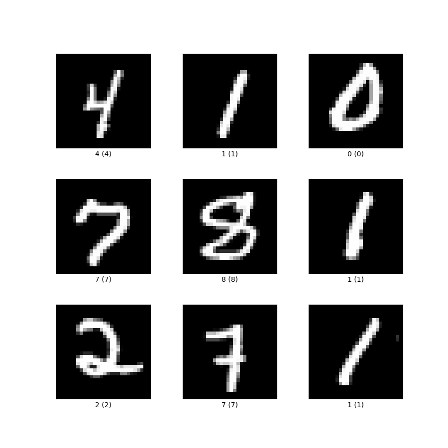
Let’s assume we’d have this input data from the MNIST data set:

So the numbers are:
4, 1, 0, 7, 8, 1, 2, 7, 1

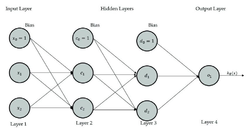
Hence the first line of the matrix X from my original image would be the 28x28 pixel greycale values of the number 4, the second line of number 1, third of number 0 and so on … each of these values multiplied by their weights and summed up would - as drawn in my image - result in the matrix Y (maybe I better should have called it marix A).

Now how do I build the second matrix? Assuming I would change the name of the matrix in my original drawing calling it A instead of Y from now on - how do I get the values for the missing matrix Y?

So would the first three lines of Y then simply be:

0, 0, 0, 0, 1, 0, 0, 0, 0, 0 (number 4)

0, 1, 0, 0, 0, 0, 0, 0, 0, 0 (number 1)

1, 0, 0, 0, 0, 0, 0, 0, 0, 0 (number 0) ?

Is that how you would “encode” the target information into the system so to say?

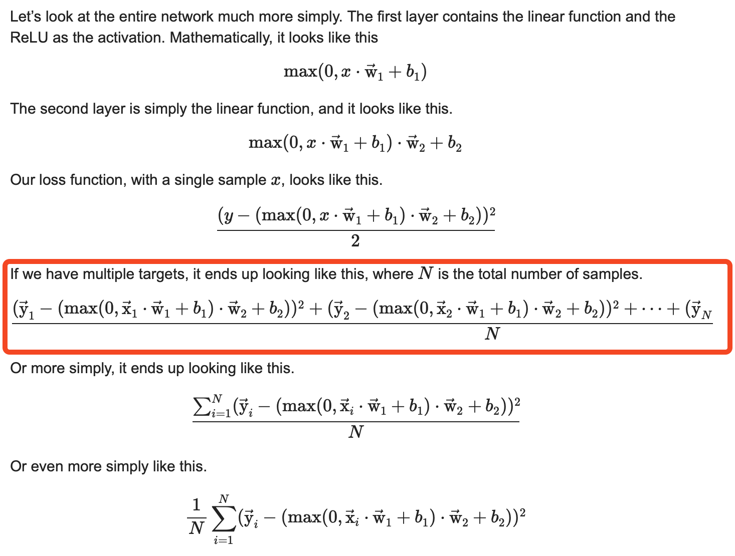
Using your notation again now we would sum up all the squared subtractions of yi - (max(0,x2⋅w1+b1)⋅w2+b2) - if we would imagine it as an animation line-wise subtracting each vector inside the two matrices line by line - and finally divide the resulting sum by the number of training examples N. Then the systems tries to reduce the error, updates the weights and gets a new error, tries to reduce it, updates the weights and so on.

Or for example in a fashion MNIST case would you then to represent a category also choose one of the 10 columns in the matrix Y? Each category one column in the matrix Y?

Say you’d have to identify 100 different cars, you’d need matrices with 100 columns - is it always like this?

Thanks again for your help, the formulas helped talking about it, very nice of you Salman! Have a good weekend everybody, see forward hearing from you

[ForBo7 (Salman Naqvi)]

So the vector \vec{\rm{y}} would be similar to the vector \vec{\rm{x}}. Just like how \vec{\rm{x}} is a vector that contains all vector data samples from \vec{\rm{x}}_1 to \vec{\rm{x}}_n, \vec{\rm{y}} contains all the corresponding scalar targets from y_1 to y_n.

The loss we’re using in the example above is MSE. So one-hot encoding the targets as you described won’t work with MSE. What would work is using the target itself. That is, the first three lines of Y would be \begin{bmatrix} 4 \\ 1 \\ 0\end{bmatrix}. To obtain the MSE for the first data sample, we would subtract the output of the network with 4, to obtain the MSE for the second data sample, we would subtract the output of the network with 1, and so on.

One hot encoding would work if we use cross-entropy loss instead.

[Laulito]

Okay now I see! So Y would then simply just be a single vector dimension N? And likewise A is more of a vector A containing the summed up elements of a single line of matrix A? Resulting in two vectors whose element-wise subtractions would need to be squared, summed up and the result would be divided by N to get the loss?

If we would use cross-entropy loss instead and the first line of Y would be
0, 0, 0, 0, 1, 0, 0, 0, 0, 0
How could we then calculate the loss assuming the first line of A would be
0.1 , 0, 0, 0.2, 0.3, 0, 0, 0.3, 0, 0.2 (just some randomness to give an example)

Thanks again for your help!

[ForBo7 (Salman Naqvi)]

We’d simply apply the formula for cross-entropy loss.

I have a guide written here that goes into how cross-entropy loss is calculated.

Let me know if you understand it.

[Laulito]

The guide is short and efficient - easy to understand and not overcomplicated unnecessarily! Great work!

Brings back memories from lesson 7 where Jeremy described the method inside an excel file! I have to admit it’s my first “iteration” watching the course, right now I’m watching episode 18 and after having watched the whole part 2 I’ll start over from the beginning, going all the way back to episode 1 is it a bird and start watching the videos again. But this time pausing the video and coding every single line by myself, diving deeper and deeper til eventually I’ll start with the third iteration of doing the course. Been very educational so far, I love it. In the first iteration I really tried to just “let it be”, trying to understand the concepts and methods rather than the code. Next time I’ll dive deeper, I promise lol.

So to get back to my example:
First line of A (preds):
0.1
0
0
0.2
0.3
0
0
0.3
0
0.2

e^preds:
1.11
1
1
1.22
1.35
1
1
1.35
1
1.22

→ SUM: 11.25

Softmax : (rounded values)
0.098
0.088
0.088
0.11
0.12
0.088
0.088
0.12
0.088
0.11

ln of softmax:
-2.32
-2.43
-2.43
-2.2
-2.12
-2.43
-2.43
-2.12
-2.43
-2.2

Actuals were 0, 0, 0, 0, 1, 0, 0, 0, 0, 0 (because it’s a 4)
So therefore the loss for the first line of the matrix would be -2.12

I guess you’d have to calculate the loss respectfully for all the other rows as well, sum them up and divide by N to get the final loss for the whole matrix. It’s always great to use actual numbers and pass them through the systems to understand their architecture. Has been very helpful, thanks again buddy