Lesson 13 official topic

Brings back memories from lesson 7 where Jeremy described the method inside an excel file! I have to admit it’s my first “iteration” watching the course, right now I’m watching episode 18 and after having watched the whole part 2 I’ll start over from the beginning, going all the way back to episode 1 is it a bird and start watching the videos again. But this time pausing the video and coding every single line by myself, diving deeper and deeper til eventually I’ll start with the third iteration of doing the course. Been very educational so far, I love it. In the first iteration I really tried to just “let it be”, trying to understand the concepts and methods rather than the code. Next time I’ll dive deeper, I promise lol.

I wouldn’t recommend doing the course multiple times. :wink:
It’d be better to start creating things and doing projects instead of staying in the theory. Doing is the only, actual way you’ll solidify your theory and gain a deeper understanding of what’s happening, and what to do and what not to do.

I guess you’d have to calculate the loss respectfully for all the other rows as well, sum them up and divide by N to get the final loss for the whole matrix. It’s always great to use actual numbers and pass them through the systems to understand their architecture. Has been very helpful, thanks again buddy

Yes, I think that sounds right. Glad to have been of help!

class Mse():

    def __call__(self, inp, targ):
        self.inp,self.targ = inp,targ
        self.out = mse(inp, targ)
        return self.out 

   def backward(self):
        self.inp.g = 2. * (self.inp.squeeze() - self.targ).unsqueeze(-1) / self.targ.shape[0]


 class Lin():

    def __init__(self, w, b): self.w,self.b = w,b
    def __call__(self, inp):
        self.inp = inp
        self.out = lin(inp, self.w, self.b)
        return self.out
   def backward(self):
        self.inp.g = self.out.g @ self.w.t()
        self.w.g = self.inp.t() @ self.out.g
        self.b.g = self.out.g.sum(0)

Shouldn’t it be self.out.g instead of self.inp.g in the backward definition of Mse class. Idk how Lin backward() automatically gets self.out.g value. Can some one explain?

1 Like

Hello,
To understand this let us first set all the code we need, then we will take it execute it step by step.
Our building blocks are:

  • the lin function: def lin(x, w, b): return x@w + b
  • the mse function: def mse(output,target): return ((output.squeeze()-target)**2).mean()
    and the classes: Mse(), ReLU(), Lin() and Model()
    Now to create our model and compute backpropagation we run the following code:
model = Model(w1, b1, w2, b2)

what happens now?:
We are calling the Model constructor so if we look inside the object model we will find:

model.layers = [Lin(w1,b1),Relu(),Lin(w2,b2)]
model.loss = Mse() 

Let’s name our layers L1, R, and L2 to make the explanation easier to follow.
so L1.w = w1, L1.b = b1, L2.w = w2 and L2.b = b2.

Now let’s execute the following line:

loss = model(x_train, y_train)

here we are using the model object as if it was a function, this will trigger the __call__ method, here is the code for it:

 def __call__(self, x, targ):
        for l in self.layers: x = l(x)
        return self.loss(x, targ)

let’s execute it:
in our case x = x_train and targ = y_train
now let’s go through that for loop: for l in self.layers: x = l(x)
the contents of model.layers is [L1,R,L2]
so the first instruction will be: x = L1(x)
similarly here again we are using L1 as function so let’s go see what’s in its __call__ method and run it:

# Lin Call method
def __call__(self, inp):
        self.inp = inp
        self.out = lin(inp, self.w, self.b)
        return self.out

so we are assigning inp to self.inp, in this case L1.inp = x_train and L1.out = lin(inp, w1,b1) = x_train @ w1 + b1.
The call method returns self.out so the new value of x will be x = L1.out.

The first iteration of the loop is done, next element is the layer R, so x = R(x)

# ReLU call method
def __call__(self, inp):
        self.inp = inp
        self.out = inp.clamp_min(0.)
        return self.out

so now we have R.inp = L1.out R.out = relu(L1.inp) # basically equal to L1.inp when it's > 0, 0 otherwise.
Now the new value of x is x = relu(L1.inp)
The second iteration is done, next element is the layer L2, so x = L2(x)
now we have L2.inp = relu(L1.inp) and L2.out = relu(L1.inp) @ w2 + b2.
The new value of x is x = L2.out = relu(L1.inp) @ w2 + b2.

The for loop has ended. Let’s go to the next line of code :slight_smile:
return self.loss(x, targ)
We saw earlier that model.loss = Mse() so we are using the __call__ method of the Mse class:

# call method of the Mse class
def __call__(self, inp, targ):
        self.inp, self.targ = inp, targ
        self.out = mse(inp, targ)
        return self.out

now we have mse.inp = x, mse.targ = targ and mse.out = mse(x, targ) = ((x.squeeze()-targ)**2).mean().
The method return mse.out so loss = mse.out.

Finally we get to the part which confused us both :smile:

model.backward()

it calls the backward method of the Model class:

# backward method of the Model class
def backward(self):
        self.loss.backward()
        for l in reversed(self.layers): l.backward()

In the first line we have model.loss.backward() which is none other than the backward method of the Mse class. because remember that loss is an instance of the Mse class.

# backward method of Mse
def backward(self):
        self.inp.g = 2 * (self.inp.squeeze() - self.targ).unsqueeze(-1) / self.inp.shape[0]

So here we compute mse.inp.g and we saw earlier that mse.ing = x so we are in fact computing x.g and it’s equal to x.g = 2 * (x.squeeze() - targ).unsqueeze(-1) / x.shape[0]

x as you know is the output of our MLP (multi level perceptron), and the gradient of the loss with respect to the output is stored in the output tensor i.e x.g. So that’s why it should be indeed inp.g and not out.g in the backward method of the Mse class.

Now in order to find out how backward of Lin get the out.g value let’s continue executing our code. We have have executed the first line now let’s run the for loop:

 for l in reversed(self.layers): l.backward()

the first value of l is L2 (because we are going through the reversed list of layers)
so let’s run L2.backward()

# Lin backward
def backward(self):
        self.inp.g = self.out.g @ self.w.t()
        self.w.g = self.inp.t() @ self.out.g
        self.b.g = self.out.g.sum(0)

We already know that:

L2.inp = relu(L1.inp)
L2.out = relu(L1.inp) @ w2 + b2 = x

so when we call L2.backward() this method will perform the following updates:

L2.inp.g =  L2.out.g @ L2.w.t() # which is equivalent to L2.inp.g = x.g @ w2.t() 
w2.g = L2.inp.t() @ L2.out.g
b2.g = L2.out.g.sum(0)

As you can see Lin knows automatically what out.g is, because when we ran model.loss.backward() we calculated it.
So now we have computed L2.inp.g (which is R.out.g) ,w2.g and b2.g.
The first iteration of the loop has ended, next l=R and we will run R.backward:

def backward(self): self.inp.g = (self.inp>0).float() * self.out.g

We know that R.inp = L1.out and R.out = relu(L1.inp)
The following updates will occur:

R.inp.g = (R.inp > 0).float() * R.out.g 

Now we have computed R.inp.g (which is L1.out.g).
This iteration is done, next is l = L1 so we will call L1.backward().
We know that L1.inp = x_train and that L1.out = R.inp
So calling backward of L1 will give us the following updates:

L1.inp.g =  L1.out.g @ w1.t() # which is equivalent to L1.inp.g = R.inp.g @ w1.t() 
w1.g = L1.inp.t() @ L1.out.g
b1.g = L1.out.g.sum(0)

That’s it.

The main takeaway is that backpropagation strats at the end and compute the gradient of the loss and stores it in the output tensor of the neural network (which is the input tensor of the loss function, and that’s what’s confusing).

I really hope that it is clear to you now, have a good day!

2 Likes

I misread your question (-‸ლ) @Senzen

I had the exact same confusion as you too, and then I eventually figured out that self.out in the Lin class and self.inp in the MSE class reference the same object; in other words, they are the same variable. That’s how self.out.g in the Lin magically gets populated.


Previous answer:
Here’s an alternative way to look at it. Let’s first look at the definition of MSE once more.

class Mse():

    def __call__(self, inp, targ):
        self.inp,self.targ = inp,targ
        self.out = mse(inp, targ)
        return self.out 

   def backward(self):
        self.inp.g = 2. * (self.inp.squeeze() - self.targ).unsqueeze(-1) / self.targ.shape[0]

What’s input is our predictions, inp, and what’s output is the loss, MSE.

A derivative tells us how one value changes with respect to another value. Take the simple equation y = mx + c. m and c are constants, whereas x is a variable. So the derivative will be with respect to x; that is, x will have the gradient.

In our formula for the MSE, our variable is our predictions which are stored in inp. Our MSE changes with respect to inp. Therefore, inp has the gradients.

Let me know if this makes sense!

1 Like

I’ve attempted to create a simple guide that explains how to derive and implement a backpropagation algorithm, by boiling down backpropagation to what it is in essence: a big chain rule equation.

The guide covers an example in a modular sort of fashion to make backpropagation easier to derive and implement, and also attempts to limit the amount of heavy notation and heavy words used.

You can read the guide here.

Do let me know of any comments, questions, suggestions, feedback, criticisms, or corrections!

3 Likes

@ForBo7 I just made an account to let you know that this went a LONG way to getting me unstuck on this. Thank you for taking the time to write this out!

1 Like

Wow! I appreciate the comment! It’s the best one I’ve received so far! :smile:

I’m glad to know my guide helped you get a better grip on backpropagation! :smiley:

Hey guys,

I still have a question that bothers me regarding the calculation of the loss of a neural network.

Assume we’d have a neural network like the MNIST one I’ve uploaded above (post # 53) that calculates an estimation for every vector x (representing the 784 pixel values of an MNIST image) inside the matrix X (that represents the sum of all 28x28 pixel images used for training). The result of that estimation / matrix multiplication can be called vector “a” and it will be stored in matrix A (although in the image in post # 53 I’ve confusingly have named the vector “y” instead of “a”).

So now to calculate the MSE loss we’d have to use the loss formula:

Loss = ((Y - A)^2) / N
which can be rewritten like pointed out by @ForBo7 like this:

Loss = ((Y - A)^2) / N = ((Y - W*X)^2) / N

And now comes the question that bothers me:
To calculate the total loss: why can’t we subtract these vectors y and a ELEMENT wise?

@ForBo7 you’ve said that for a MSE loss the first three lines of Y would be
(4,
1,
0)
but why couldn’t it be

(0, 0, 0, 0, 4, 0, 0, 0, 0, 0
0, 1, 0, 0, 0, 0, 0, 0, 0, 0
0, 0, 0, 0, 0, 0, 0, 0, 0, 0) ?

I thought about this when I’ve looked at the neurons on the right side in the image in my post (post#53). Assuming their activations would produce a result that would sum up to the exact same numbers (4,1,0,…) but would be placed on a wrong position then the loss would be 0 although the model would have predicted the result totally wrong.

Speaking in numbers instead of words:
If A would be:
(4, 0, 0, 0, 0, 0, 0, 0, 0, 0 Σ = 4
0, 0, 0, 0, 1, 0, 0, 0, 0, 0 Σ = 1
0, 0, 0, 0, 0, 0, 0, 0, 0, 0 Σ = 0)

Then the loss L=(y-a)^2 would be 0 because the elements would sum up to the same value although being in the wrong place / in the wrong neurons.

Can someone explain to me why we sum the vectors up before computing the loss? How would that avoid the above issue?

And is there some more in depth explanation / literature / book that connects the different types of mathematical loss equations with the network architecture of the neurons in a neural network?

Firstly, and most importantly, I love, love, love this course (and the previous one!)

However, from the perspective of a professional Python software engineer, most of the Python presented is pretty weird/ugly. It kinda came to a head with the abstract-class-based Model implementation in this lesson. So I fixed it :smiley:

class Module:
    def __call__(self, *args: Tensor) -> Tensor:
        self.input_ = args[0]
        try:
            self.target = args[1]
        except IndexError:
            pass
        self.output = self.forward()
        return self.output

    def forward(self) -> Tensor:
        raise Exception("not implemented")

    def backward(self) -> None:
        raise Exception("not implemented")


class Relu(Module):
    def forward(self) -> Tensor:
        return self.input_.clamp_min(0.0)

    def backward(self) -> None:
        self.input_.g = (self.input_ > 0).float() * self.output.g


class Lin(Module):
    def __init__(self, weights: Tensor, biases: Tensor) -> None:
        self.weights, self.biases = weights, biases

    def forward(self) -> Tensor:
        return self.input_ @ self.weights + self.biases

    def backward(self) -> None:
        self.input_.g = self.output.g @ self.weights.T
        self.weights.g = self.input_.T @ self.output.g
        self.biases.g = self.output.g.sum(0)


class Mse(Module):
    def forward(self) -> Tensor:
        return (self.input_.squeeze() - self.target).pow(2).mean()

    def backward(self):
        self.input_.g = (
            2 * (self.input_.squeeze() - self.target).unsqueeze(-1) / self.target.shape[0]
        )

The primary changes here are:

  • using class/instance attributes (by assigning from __call__()'s *args) instead of passing the same values as method parameters.
  • Descriptive variable names - this one gives me palpitations, especially when reading ML/AI source; I guess it’s because most authors come from a Mathematics background :person_shrugging:

The amount of difficulty I had in chasing the various args through the code (I think) perfectly demonstrates why going “all in” on OOP is better than mix-and-matching. RIght up until I ran everything and verified the results I wasn’t even sure I had refactored it correctly :sweat_smile:

The Module class obviously has a little bit of magic for de-marshalling *args, but I still find the result more readable/intuitive. If this were a much larger example (in terms of number of subclasses of Module), I’d try to find a different architecture. In any case, TL;DR - if you don’t like self, don’t do object-oriented Python :smile:

I’ve also added type annotations where possible (NONE of the type checkers I tested understood typing a dynamic attribute, i.e., the .g we use for storing the backprop gradient, although it is valid per the relevant PEP)

Fantastic lecture again!

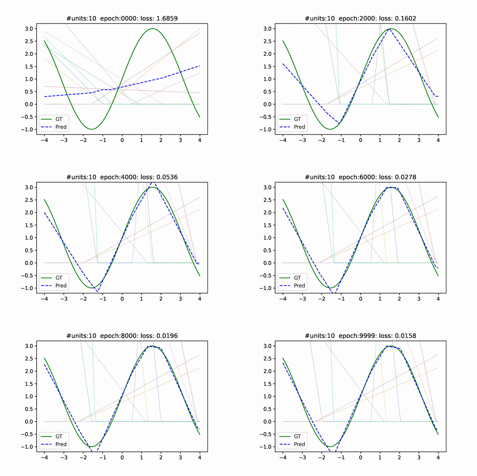
I have created a notebook to demonstrate the use of rectified linear units to match any arbitrary curve. I tried to recreate the diagram that Jeremy drew in the video.

Notebook
20240503_relu_stepbystep.ipynb

Summary
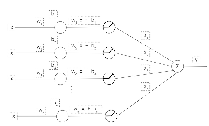
The goal is to approximate any 1D curve of the form y = f(x) where x and y are scalars. To accomplish this, I attempt to learn the slope and intercept (weight and biases) of ‘n’ lines. I then pass the output through a ReLU function and perform a weighted sum to predict y. In our model (figure below), wi’s, bi’s and αi’s are learned using MSE loss.

Results

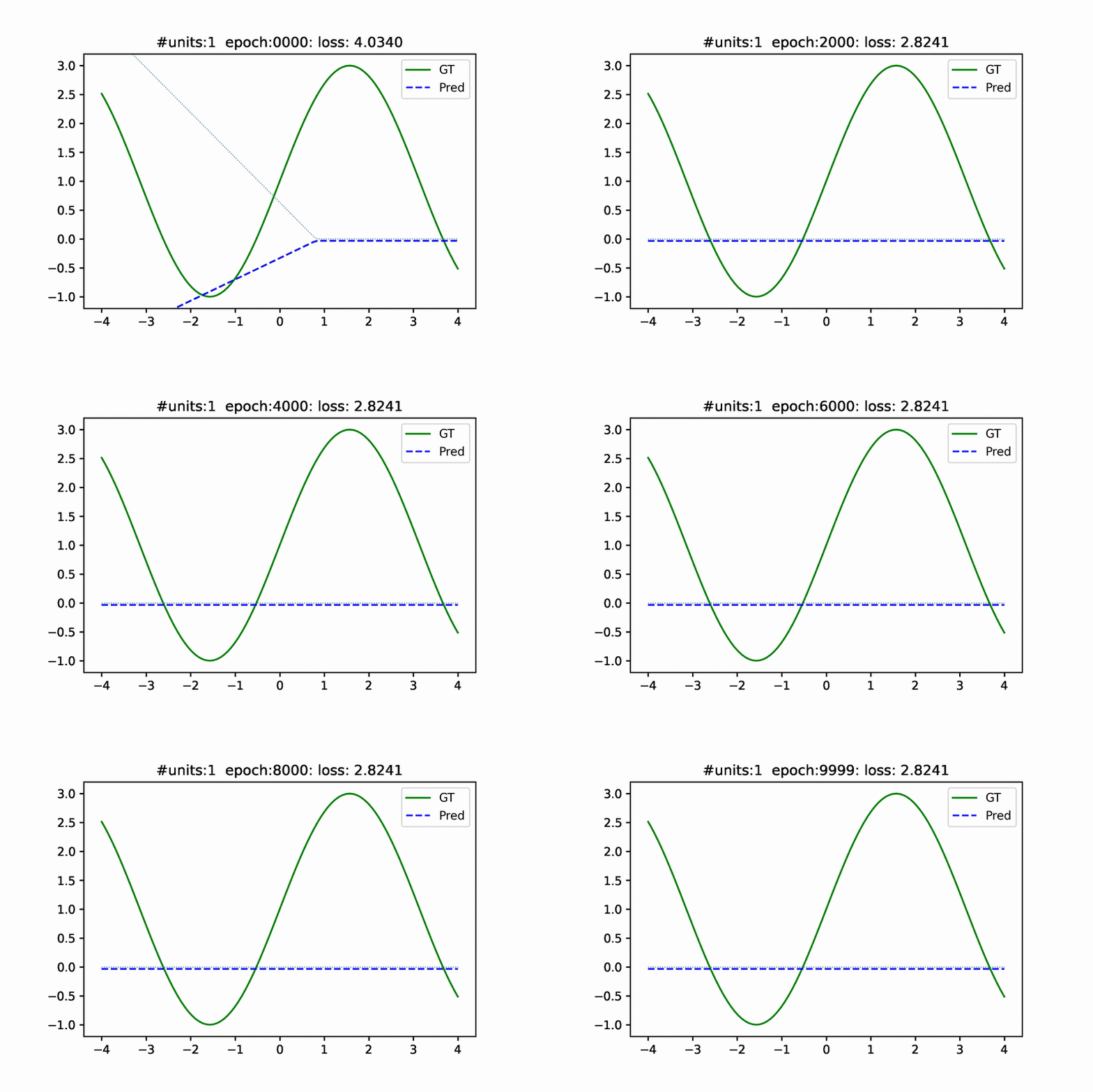
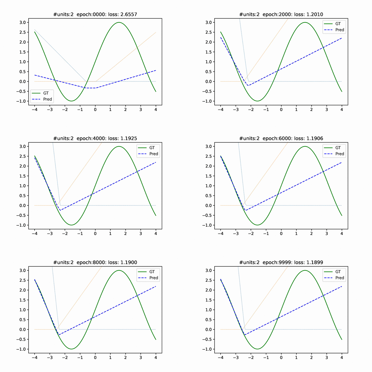
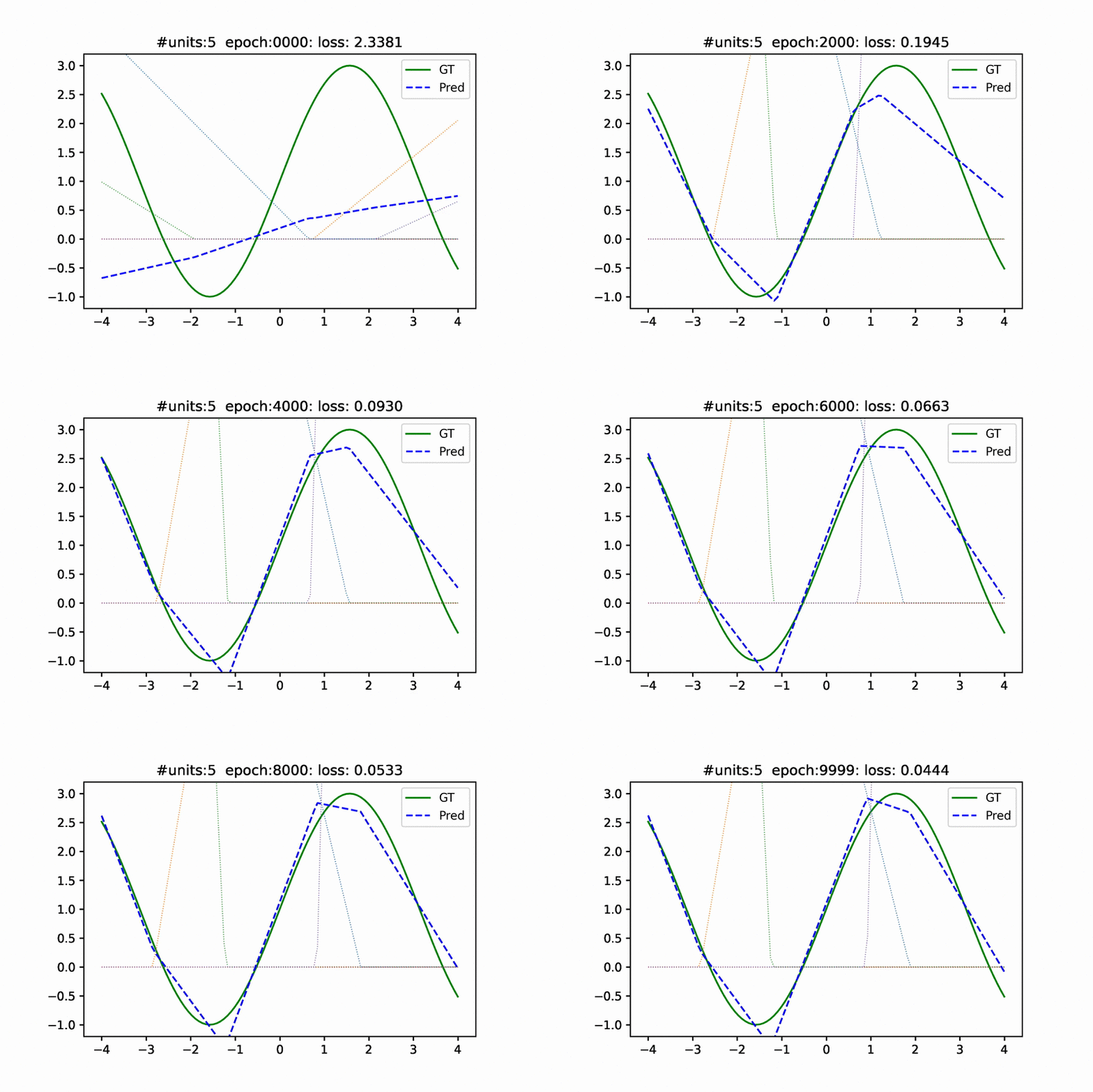
Following GIFs shows how, over training iterations, this simple network is able to approximate the curve. In the GIFs the faint lines represent wi * x + bi after applying ReLU. The dotted blue line is the weighted sum of these lines (prediction). The solid green line is the curve that we are trying to approximate (ground truth or GT). The four plots correspond to using 1, 2, 5 and 10 units.

ReLU Curve Fitting 1 Unit ReLU Curve Fitting 2 Units
ReLU Curve Fitting 5 Units ReLU Curve Fitting 10 Units
1 Like