Lesson 13 official topic

The most important things to do IMO is ensure you’ve got the pre-reqs - i.e. watch the 3blue1brown ‘essence of calculus’ series and enough of Khan Academy that you’ve covered derivatives and the chain rule. If you didn’t cover that in high school (or did, but have forgotten it), then you’ll need to back-fill that stuff now, and the fast.ai material in lesson 12 won’t make that much sense without it (since we’re starting on the assumption that you’re already comfortable with that).

It’s not any harder than anything else we’ve done up until now in the course, and I’m sure you’ll be able to pick it up with time and practice! I’ll create a new thread for asking calculus questions now - feel free to use it to ask anything you like.

4 Likes

OK here’s the topic:

2 Likes

Folks, in case it proves helpful to anyone, see link below for my rough attempt to connect the code and the math in the 03_backprop.ipynb notebook.

9 Likes

This is a really nice piece of work, thanks for sharing, I have been doing a similar thing but yours is much better layed out

Thanks for the encouragement @johnri99!

I was trying to work through some backprop on pen and paper this past week (along with the code)
and always got a little stuck when I got to higher order Jacobian stuff. I mean the layers in the middle where you have dY/dX and both are tensors and not like a simple scalar loss. I was expressing some of my confusion in one of the study groups and someone recommended this video. It has has some nice heuristics and explanations on how we get those results without computing the entire Jacobian. This was a video that made it make more sense to me. It’s another example of “getting the shapes to work out” which is a theme that keep coming up (broadcasting etc.) Just sharing the link to the video in case anyone else was stuck on similar thing.

9 Likes

This was fantastic! Thank you!

Same here Alex. In addition to the suggestions above, this helped me a lot: Make Your Own Neural Network
also, I watched the V3 version of the second part first (2020) and watched this lesson again. V3 is essentially the same as this, but I believe both are complementary. A slightly different angle to the same thing is very helpful.

2 Likes

This link clearly explains the result:

http://cs231n.stanford.edu/handouts/linear-backprop.pdf

4 Likes

I read this over the weekend and can confirm that it’s quite useful at this low level stuff. Esp going end to end with some simple networks, showing how the various pieces fit together and so on. Filled in some gaps in my understanding, for sure. Thank you for the recommendation, @nikem!

1 Like

That’s great to see so many good explanations of backprop and chain rule. Kudos to @sinhak for writing this down for matrix case! It is not the first time I approach chain rule and trying to implement it from scratch. However, deriving partial derivatives and Jacobians, especially, for multiple layers, has always been a struggle. (And still is, actually…)

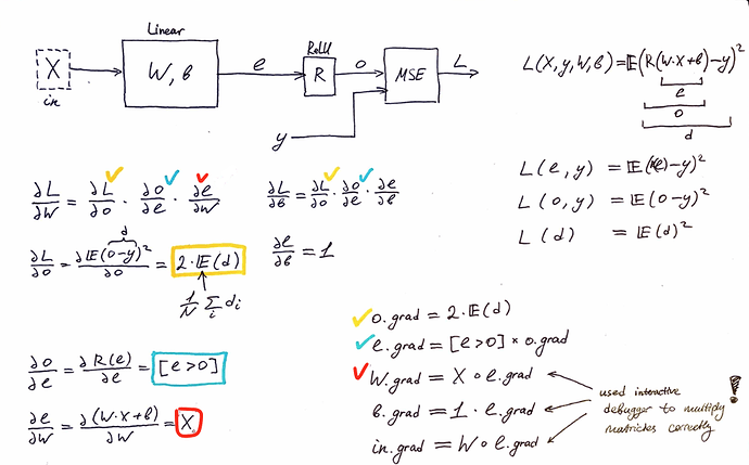
This time, I tried to use Jupyter and PyTorch as “copilots”: I started with pen and paper, but figured our the right multilications using pdb. Here is my small note with somewhat trivial derivations, but it helped me to reimplement forward/backward path for linear layers “from scratch”; and it was great to see that my implementation is aligned with what was presented during lectures. (Except that I don’t sum up the last dimension for bias tensor, and keep it as a “column” vector.)

Essentially, I derived the equations for scalar case, and tried to align the shapes of gradients with the shapes of weights, i.e., if W is 4x3, then W.grad should have the same shape in order to do an update. And, it worked! So, an interactive playground is great assistance in this. As well as autograd frameworks that you can use to check if everything is done correctly.

I wonder if it is possible to do the same for conv/attention layers? Like, starting with somewhat lousy math and figuring out the right implementation using interactive playground. Might be an interesting learning experiment.

3 Likes

Yet another presentation about the gradients of transformations and backpropagation - while the concept of derivatives is simple for functions of one argument, making it work for multi-dimensional data requires advanced linear algebra skills and it is better to trust PyTorch :slight_smile:

In my newly created Quarto blog to support my learning I added a post about Derivatives and chain rule.

2 Likes

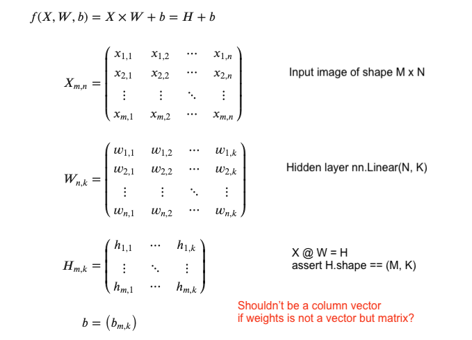
By the way, I just realized that I don’t quite understand why the bias is a vector and not a matrix in PyTorch’s implementation. (See the following snippet.)

    # torch.nn.Linear
    def __init__(self, in_features: int, out_features: int, bias: bool = True,
                 device=None, dtype=None) -> None:
        factory_kwargs = {'device': device, 'dtype': dtype}
        super(Linear, self).__init__()
        self.in_features = in_features
        self.out_features = out_features
        self.weight = Parameter(torch.empty((out_features, in_features), **factory_kwargs))
        if bias:
            # bias is a vector?
            self.bias = Parameter(torch.empty(out_features, **factory_kwargs))
        else:
            self.register_parameter('bias', None)
        self.reset_parameters()

Looking at the equation, I expected that, in general, it might be a matrix:

X • W + b
^   ^   ^
|   |   |
|   |   should be of shape (n, k)?
|   |
|   this one might be (m, k), right?
|
say, this one is (n, m)

Does it broadcast the bias vector in cases when linear matrix multiplication returns a matrix?

Hehe. Everything you ever learned in math class is now wrong thanks to broadcasting. Jokes aside, this kind of stuff gets me all the time because I first learned this stuff from strict math point of view.

1 Like

Bias is a vector with number of elements equal to the number of output features (as you see in the code). So for each sample (row of X) the bias is the same. If there are many samples in a batch then the bias is broadcasted. If there is a single output than the bias is a single number.

1 Like

Yeah, I understand this part for the case when we have a system of linear equations, like:

| x11 x12 x13 |    | w1 |   | b1 |   | x11*w1 + x12*w2 + x13*w3 + b1 |
| x21 x22 x23 | x  | w2 | + | b2 | = | x21*w1 + x22*w2 + x23*w3 + b2 |
| x31 x32 x33 |    | w3 |   | b3 |   | x31*w1 + x32*w2 + x33*w3 + b3 |

However, I wasn’t sure if that works the same way in cases when we have a matrix of weights, and not a column vector. So, it means that we model bias in such a way that each coefficient is broadcasted across the columns, right?

Somehow, I thought that it is more like the following picture shows.

matmul

But I guess I just didn’t get the equation right and mistakenly generalized it from the lower dimension. Good to know!

Nice easy to read article. Elegant use of matrix transposition rules (which I had to look up.) I like your graphic representing loss as a combination of the last layer.

I don’t quite get the idea of differentiating the weights, and their gradient is equal to the input. Within a forward & backward pass, aren’t the weights constant? …and only updated between passes?

Extract…

Thank you, @bencoman :slight_smile:

About the differentiation - if w is viewed as a variable and x as a constant then the derivative of y with respect to w is x - the same logic as for the case of dy/dx.

In the forward pass we calculate the output and the loss. In the backward pass we calculate the gradients with respect to the weights and we save them. So we calculate if we change the weights how much the output y and finally the loss will change. You are right - the weights are updated between the passes.

Or I misread the question?

1 Like

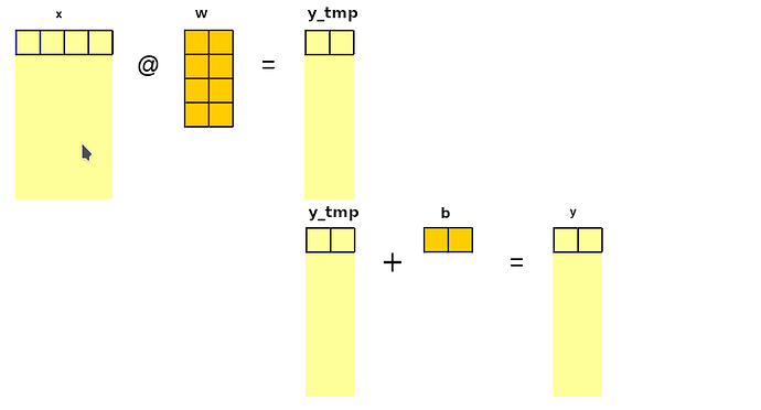
May be the confusion comes from the input array content interpretation. For fully connected networks the input is not an image but a batch of vectors, each vector containing single input - could be an image but flattern from 2D to 1D. May be the next image will explain why we need to broadcast the bias. The same way the weights matrix does not change if the size of the batch is changed, the bias can’t change its shape with the change of the batch size and shoud be broadcasted. So x W + b for undefined batch size looks like:

1 Like

I have added some outputs (within 03_backprop.ipynb) and simplified training set to dum it down as much as possible and track every single step happening on forward&backward pass. It helped me a lot! Here it is:

# dummy training set
x_train = tensor([[1.0,0.0,0.0,0.0,0.0,0.0,0.0,0.0,0.0,1.0],
                  [1.0,0.0,0.0,0.0,0.0,0.0,0.0,0.0,0.0,1.0],
                  [1.0,0.0,0.0,0.0,0.0,0.0,0.0,0.0,0.0,1.0],
                  [0.0,0.0,0.0,1.0,0.0,1.0,0.0,0.0,0.0,0.0],
                  [0.0,0.0,0.0,1.0,0.0,1.0,0.0,0.0,0.0,0.0],
                  [0.0,0.0,0.0,1.0,0.0,1.0,0.0,0.0,0.0,0.0],
                  ])
y_train = tensor([1,1,1,0,0,0])
x_valid, y_valid = x_train[:5], y_train[:5]

# predefined simple initial weights so you can track calculations
w1 = tensor([[1.0, 0.],
            [1., 0.],
            [-1., -1.],
            [-1., 1.],
            [-1., -1.],
            [0., 0.],
            [-1., 0.],
            [0., 0.],
            [-1., 0.],
            [0., 0.],])
b1 = torch.zeros(nh)
w2 = tensor([[-1.0],
            [ 1.0]])
b2 = torch.zeros(1)

### [...]

# and finally two main functions modified with some output
def lin_grad(inpt, outpt, ww, bb, inpt_n, outpt_n, ww_n, bb_n):
    print("*lin_grad(inpt, outpt, ww, bb)*")
    # grad of matmul with respect to input
    print("{}.t:".format(ww_n),ww.t())
    inpt.g = outpt.g @ ww.t()
    print("~~~{}.g = {}.g @ {}.t():".format(inpt_n,outpt_n,ww_n),inpt.g)
    #print("{}.unsqueeze(-1):".format(inpt_n),inpt.unsqueeze(-1))
    ww.g = (inpt.unsqueeze(-1) * outpt.g.unsqueeze(1)).sum(0)
    print("~~~{}.g = ({}.unsqueeze(-1) * {}.g.unsqueeze(1)).sum(0):\n".format(ww_n,
                                                                    inpt_n, outpt_n)
                                                                                  ,ww.g)
    bb.g = outpt.g.sum(0)
    print("~~~{}.g = {}.g.sum(0):\n".format(bb_n,outpt_n),bb.g)
    return ww.g, bb.g

def forward_and_backward(inp, targ):
    # forward pass:
    l1 = inp @ w1 + b1
    print("l1 = inp @ w1 + b1:",l1)
    l2 = relu(l1)
    print("l2 = relu(l1):", l2)
    out = l2 @ w2 + b2
    print("out = l2 @ w2 + b2:", out)
    diff = out[:,0]-targ
    print("diff = out[:,0]-targ:", diff)
    loss = diff.pow(2).mean()
    print("\n**** !!! loss = diff.pow(2).mean():", loss)
    #pdb.set_trace()
    
    # backward pass:
    print("\n***backward pass***")
    out.g = 2.*diff[:,None] / inp.shape[0]
    print("out:",out)
    print("out.g = 2.*diff[:,None] / inp.shape[0]:",out.g)
    print("\n*working on l2*")
    print("lin_grad(l2, out, w2, b2):")
    w2_grad, b2_grad = lin_grad(l2, out, w2, b2,
            inpt_n="l2",
            outpt_n="out",
            ww_n="w2",
            bb_n="b2")
    print("\n*working on l1*")
    print("(l1>0).float():",(l1>0).float())
    l1.g = (l1>0).float() * l2.g
    print("l1.g = (l1>0).float() * l2.g:",l1.g)
    print("lin_grad(inp, l1, w1, b1)")
    w1_grad, b1_grad = lin_grad(inp, l1, w1, b1,
            inpt_n="input",
            outpt_n="l1",
            ww_n="w1",
            bb_n="b1")
    return w2_grad, b2_grad, w1_grad, b1_grad

# call it 
w2_grad, b2_grad, w1_grad, b1_grad = forward_and_backward(x_train, y_train)

# and you can also make another call after updating weights and see how loss changes
lr = 0.5
w1 = w1 - w1_grad*lr
b1 = b1 - b1_grad*lr
w2 = w2 - w2_grad*lr
b2 = b2 - b2_grad*lr

Hope this can help someone as helped me.
2 Likes