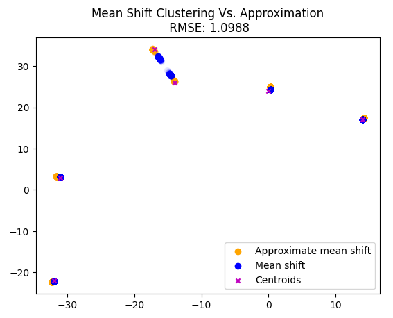
I took a crack at inventing a new meanshift algorithm which picks only the closest points, to avoid quadratic time. I got a ~40% speed increase over the initial cpu implementation with an RSME of 1.0988 compared to the original algorithm results.
My approach was to only evaluate points around the same radius (or the same vector length for an n-d arrays).
Step 1: calculate vector length
Step 2: sort the new array by vector length
Step 3: calculate the approximate number of indices to look around.
Step 4: perform mean shift weighting on subset of data
Step 5: update the array
To find how many indices to look around I counted the number of points in a histogram bin where the bin was the bandwidth range (2bw) multiplied by the number of standard deviations specified (n_std). I originally used 6 sigma but got getter results with 7.
X = data.clone(); bw=2.5; n_std=7

def clamp(n, smallest=0, largest=len(X)-1): return max(smallest, min(n, largest))

for it in range(5):
    vec_len=torch.sqrt((X**2).sum(axis=1))
    X_sorted, indices = torch.sort(vec_len)
    bin_cnts=torch.histc(X_sorted, bins=int(torch.ceil(X_sorted.max()-X_sorted.min()/(2*bw*n_std))),
                     min=X_sorted.min(), max=X_sorted.max())

    search_tol=int(torch.ceil(bin_cnts.std()*n_std))
    for i, idx in enumerate(indices):
        lw=i-search_tol
        up=i+search_tol
        x=X[idx]
        X_sec=X[indices[clamp(lw): clamp(up)],:]
        dist = torch.sqrt(((x-X_sec)**2).sum(1))
        weight = gaussian(dist, bw)
        X[idx] = (weight[:,None]*X_sec).sum(0)/weight.sum()
Approximate Meanshift time: 888 ms ± 16 ms per loop (mean ± std. dev. of 7 runs, 1 loop each)
Regular Meanshift time: 1.26 s ± 49.5 ms per loop (mean ± std. dev. of 7 runs, 1 loop each)
I also thought comparing the usual img2img pipeline with a pipeline where the prompt is an image and it is done in several steps with the diffusion loop. But, as you said, the problem is that the text encoder uses generates (lenght_of_prompt, 768) hidden states while image encoder generates (257, 1024) hidden states.
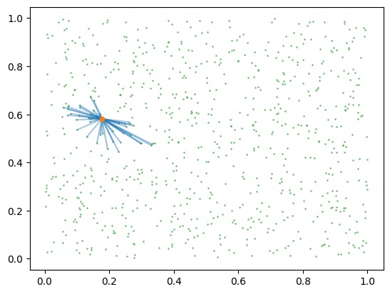
TIL about locality-sensitive hashing! What a cool technique for limiting the search size for this kind of problem, and super easy to implement in PyTorch. For ref, I found this blog post a really great resource as it went through what the hashing function could actually be - and the fact that it’s just some linear projections plus a floor function to create bins fits so nicely with PyTorch! (very reminiscent of NNs in that it’s just a randomly initialised matrix multiplication + a non-linearity)
import torch
import matplotlib.pyplot as plt

dim = 2
uniform_data = torch.rand((800, dim))

n_hashes = 40

# The actual hashing function
# really, each hash should be the first component of a rotation matrix + a bias
# but this approach seemed to work ok too. I suspect it's too dependent on tuning
# the hyper params in higher dimensions, though
H_matrix = torch.rand((dim, n_hashes))
m_factor = 5
def h(x):
    return (x @ H_matrix * m_factor).floor()

hashed = h(uniform_data)

random_point = torch.rand((dim))

# More collisions -> closer
n_collisions = (h(random_point) == hashed).sum(dim=1)

# Plot lines between our random point and points in our dataset that have a lot of collisions.
for n, point in zip(n_collisions, uniform_data):
    if n <= 30:
        continue
    plt.plot(
        *torch.stack([random_point, point]).T,
        alpha=n.item() / n_hashes * 0.5,
        color="C0",
    )


plt.scatter(*uniform_data.T, s=1, alpha=0.5, color="C2")
plt.scatter(*random_point.T, s=20, alpha=1, color="C1", zorder=3)
I used this with k-means, but it makes it even more sensitive to the initial choice of centroids, because its very possible the some of the points in a different cluster aren’t close enough to an initial centroid. I think it would work super well with algorithms like DBSCAN and mean shifting though, because they already rely on calculating distance from each point and looking at the closest.
The einstein summation notation in the lesson looks different than the one I remember from physics,
in physics, if we have a variable repeated in both matrices then this variable is called a dummy variable that is summed over so Aik x Bkj = Cij. Correct me if I’m wrong but i thought it is a way to reduce the shape of the tensor not the opposite.
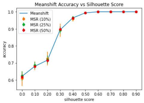
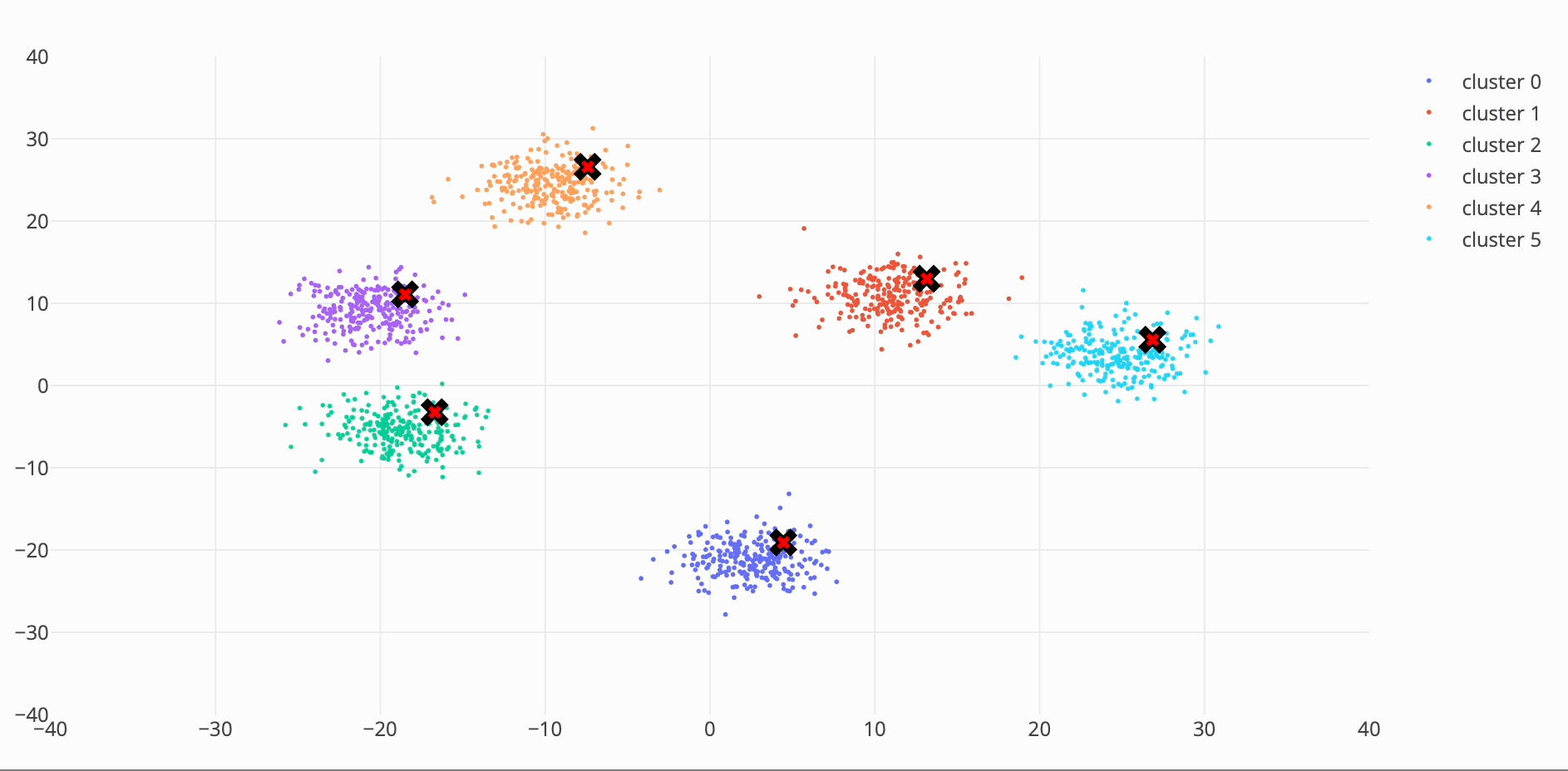
@jeremy I ran some experiments to figure out when meanshift with random sampling (MSR) is as accurate as the naive meanshift algorithm.
Figuring out this when is a pretty big open-ended problem so to keep things simple (and hopefully useful) I generated a bunch of synthetic datasets with silhouette scores ranging from 0 => 1.
Sidebar: Datasets with dense, well separated clusters have a high silhouette score, while datasets with overlapping clusters will have a lower score. Datasets can have a silhouette score as low as -1 when the clusters are incorrect. Datasets with scores < 0 were not considered as I didn’t think they were particularly useful for this experiment.
The plot below shows the accuracy of 3 MSR variants w.r.t the naive meanshift algorithm on datasets with silhouette scores ranging from 0 => 1. We can see that even 10% MSR produces competitive results for datasets with a silhouette score > 0.5.
Note: The error bar for a particular silhouette score and algorithm was generated by running the given algorithm (e.g. MSR 10) from scratch 50 times and then computing the standard deviation of the accuracy.
As a sanity check I ran a similar experiment on the well known UCI Breast Cancer Wisconsin dataset which has a silhouette score of 0.57. The results are summarised in the table below:
Algorithm
Accuracy
Meanshift
0.93 \pm 0.00
MSR (10%)
0.92 \pm 0.03
MSR (25%)
0.93 \pm 0.01
MSR (50%)
0.93 \pm 0.00
Although this analysis only scratches the surface it appears that meanshift with random sampling provides a significant boost in performance (up to 4x) with only a minor drop in accuracy for datasets with a silhouette score > 0.5.
In particular, MSR 25% seems to strike a nice balance between performance (~3.5x improvement) while still producing competitive results.
Hello,
First of all, thank you so much Jeremy for such a wonderful and thorough course, and for your generosity sharing your knowledge and expertise, both theoretical and practical. I am learning a lot and feel really grateful, and I regret that I waited so long before exploring your courses.
Then, I have a question regarding the implementation of function one_update() in this lesson. The function modifies tensor X inside its loop. So, after each iteration, when the next data point is measuring its distance to all other data points, it sees updated values for data points that were processed before it, instead of seeing their initial values (at the start of the loop). When I change the code to use an extra tensor to store the updated data in, the animation runs slower.
I’m not quite sure if this is a bug in the code (perhaps a benign one that does not change the final result, but speeds up the convergence), or if this is an intentional optimization, since it doesn’t matter if one uses the original data or updated data for subsequent rows.
And by using vmap from torch.func, one can very easily use the one_update function from the lesson written for updating one sample to apply it over mini-batch or whole batch without having to deal with the correct shapes for batched case and with equivalent performance of hand vectorised code.
import torch
import math

def gaussian(d, bw): return torch.exp(-0.5 * ((d / bw))**2) / (bw * math.sqrt(2 * math.pi))

def update(x, X):
    # x -> sample
    # X -> data
    dist = torch.sqrt(((x - X)**2).sum(1))
    weight = gaussian(dist, 2.5)
    return (weight @ X) / weight.sum()

# Random Data
X = torch.randn(1500, 2)

# for-loop version
results = []
for i in range(100):
    results.append(update(X[i], X))

expected = torch.stack(results)

# vmap version

# vmap only over sample and not the complete data.
actual = torch.func.vmap(update, in_dims=(0, None))(X[:100], X)

# Sanity Check
torch.testing.assert_close(actual, expected)
Mean shift in jax. Was not aware of the new vmap functionality in PyTorch, very nice! I prefer building up from non-vectorized to vectorized via vmap instead of broadcasting!
At about 51:40 Jeremy says a bandwidth that covers about 1/3 of the data is a good choice i.e. brought two clusters. He then chooses a value of 2.5. Why that? It looks more like the value 25 would be a better choice, doesn’t it?
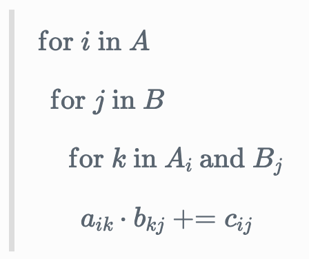
I created a guide to more intuitively understand and use Einstein summation notation, as I found the quick rules to use it confusing.
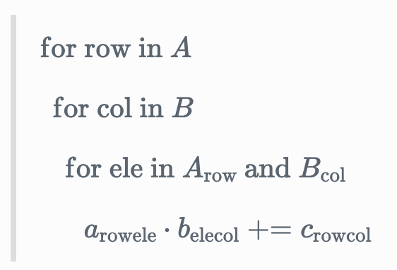
Matrix multiplication in einsum notation is written is ik, kj \rightarrow ij. The key to understanding this is to not think of i, j, k as axes, but rather as iterators.
Matrix multiplication simply involves taking the dot product of each row in the first matrix with each column in the second matrix.
We’ll need to use 3 iterators for this: one iterator i to loop through the rows of A, another iterator j to loop through the columns of B, and a third iterator k to loop through the elements in a row and column.
If we focus on the last line above…
a_{ik} \cdot b_{kj} \mathrel{+}= c_{ij}
…this can more succinctly be written in einsum notation as ik, kj \rightarrow ij — for each row i in A, and for each column j in B, iterate through each element k, take their product, and sum those products. The location of the output of the dot product in the output matrix C is c_{ij}.
You can read through the full guide with more examples with the link below.
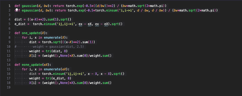
Calculating mean-shift using Pytorch einsum.
(My apologies for the previous post I had forgotten to include some of the code)
I can’t remember where in the pytorch docs or StackOverflow I saw the inspiration but, I found an interesting way to use numpy matrix multiplication within the einsum() function. I’ve paired the traditional way to calculate the mean-shift algorithm with the einsum() version.
I think it depends on the algorithm (k-means, DBSCN,…) you are working on.
In my case, 30 min to make k-means to work.
The video animation part took more time though
I go over the algorithm, some python code implementing it from scratch, and two basic experiments. Additionally, I wrote a Colab notebook where you can play around with some of the code and experiments yourself.
This is my first blog post; so it’s nice to get started with this course.