I appreciated Jeremy’s explanation of how neither Prompt->Image nor Image->Prompt are invertible functions. But perhaps we can devise an approximate inverse, one that given an image finds a prompt that generates a similar image, and does it better than Clip Interrogator.
Suppose we get the latents for the source image. The image generator has been trained with contrastive loss to match the CLIP caption latents to their image latents. Therefore the image latents should be near to the latents made by some as yet unknown prompt.
Next, optimize the CLIP input embedding itself using gradient descent, keeping CLIP’s weights frozen, to find an input embedding that generates something close to the image latents. This yields an input text embedding.
(You cannot go all the way to an input prompt because a vocabulary is not continuous.)
Next, invert the text embedding to a language prompt. This is not straightforward. Certainly not all (if any) of the word embeddings will map back to a specific word - a word embedding may represent a mixture of word concepts. Still, you could try mapping the word embeddings to the nearest word embedding in CLIP’s vocabulary. Or look for a combination of word embeddings, like a hyphenated term, that produces something near to the target word embedding. My hope is that the phrase would map through CLIP close to the original image latents.
So there you have it, with a good deal of hand waving. Issues I see…
Can the layers of transformers in CLIP be reversed to find a text embedding? I do not understand well enough how CLIP works to answer with certainty.
You may need to add back in the image latents of the empty prompt before training to find the text embedding.
Mapping word embeddings back to a phrase (approximately) is tricky. It’s a paper in itself!
It may generate nonsense, like a string of “end-of-sentence”. Or many “concepts” for which we have no English word.
Why don’t I do it myself? I am not smart enough! Someone familiar with the code could test this idea in an hour, while it would take me many days to do so.
If someone also likes a little slower version of meanshift, the animation was a bit too fast for my liking so i added a learning rate to one_update() to scale the shifting
Jeremy mentioned that we could improve the efficiency of the meanshift algorithm by only considering the nearest points when computing the weighted average.
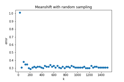
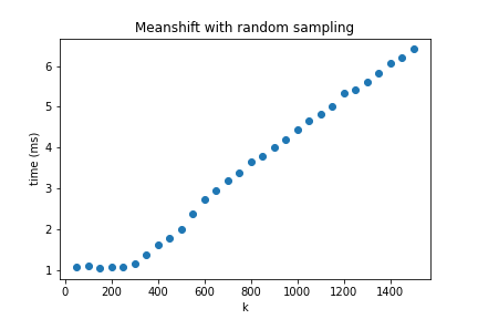
I was curious to see how a more naive solution would perform. Instead of picking the k nearest points when computing the weighted average why not pick k points at random?
The plot below shows error as a function of k where error is defined as the average distance (euclidian) between each point in the dataset and its known centroid after 5 meanshift iterations. As a reference the baseline error of the dataset is ~3.62. As you can see once k is ~5% of the dataset the error rate is pretty reasonable.
This is an O(nk) solution and for k << n this becomes an O(n) solution. Whether k = 5% of n counts as k << n in this context is debatable (it probably doesn’t). I suspect this naive approach would fall apart on more challenging datasets with higher dimensions and class imbalance.
Note: Aside from the random sampling the only change I made to the lesson12 notebook was the addition a small bias of 0.0001 to the tri method. When the weighted average is based on random samples its possible that all samples will be too far away resulting in a weight matrix of all zeros. The bias ensures the weight matrix will be non-zero.
Here’s an animation which shows how the dataset shifts as a function of k.
I implemented K-Means in pytorch trying to remove as many loops as I could and sticking to pytorch tensor functionality and posted in on my new quarto blog. The broadcasting applied to a new problem was really good practice for me, as well as reading what k-means is in math language and translated it to code.
There’s still 2 loops that I haven’t figured out how to remove. One is in the centroid initialization and I don’t think that can be removed with the initialization strategy I went with (it’s the one that made the most sense to me).
The second is a loop that I think should be removable in the update_centroids function, but I haven’t figured out how to get rid of it yet. If anyone has any ideas, I’m all ears!
I did k-means, too. It’s simple enough but it was very valuable working those tensor manipulation muscles. I’m hoping to implement another one of the algs JH mentioned, too.
For my part, I produced an animation of k-means in action, with 10m data points generated each time. You can really see how efficient the algorithm (in terms of steps) and its common failure modes. (The predicted means were intialized to an existing data point pickeed at random.)
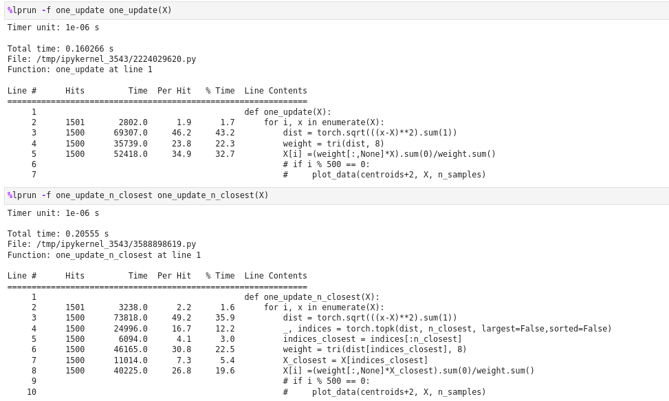
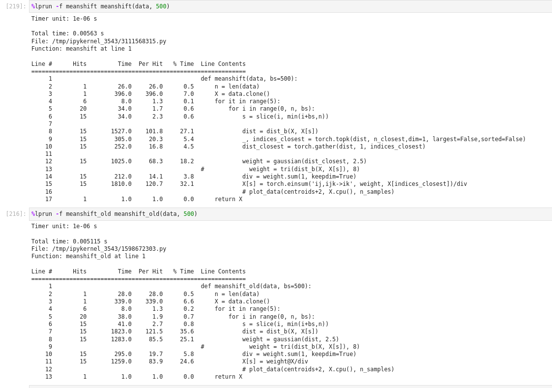
Anyone succeeds to implement the new meanshift that picks only some closest points? I’ve tried both for the no batching and batching but can not make it faster than the original one.
For no batching, the function to pick the closest points takes too much time, so can’t compensate for the gain from matrix multiplication
For the batching one, not sure if my implementation is correct, but it is no more the matrix multiplication because each point has a different set of n_closest points. This means instead of [batch x n_points] x [ n_points, 2 ] we now have [batch x n_closest_points] x [n_closest_pointsxbatchx2] and the excecution time is higher than the original one.
You need an approach to approximately finding the closest points that is faster than O(n) – i.e. super-linear. For instance, locality sensitive hashing, ball tree, kd tree, octree, etc.
Like others, I also picked kmeans to practice some broadcasting and so on.
I was reminded how important the centroid initialization is. First I went for the simplest approach
which picks k centroids at random. But this often leads to subpar results like this:
I then went for a different initialization scheme motivated by kmeans++ where you pick the initial centroids in such a way that they are more spread out. It worked better. You have to do some more computation upfront before the iterations but the convergence is much quicker after. And the results are usually better too. Like this:
I still need to practice broadcasting a lot more and it still seems like magic to me in some cases.
I’m still surprised that this code snippet does the pairwise distances between all pairs of vectors in two 2D tensors:
# broadcasted version of squared Euclidean distance
def square_distance(Xb, Xq):
    return (Xb[:, None] - Xq[None]).square().sum(2)
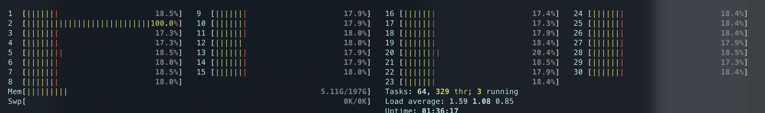
When I was debugging my code initially I was curious to why it was running sort of slow. It turned out
that part of my code was not running on the GPU but was still on the CPU. I actually found using htop to be useful in visualizing what the cpu and memory were doing. It looked way to busy and then I knew something was wrong b/c the GPU should have been doing the heavy lifting. Turns out my weighted sampling for the more clever initialization was still running on the cpu device instead of gpu. So good tip to check htop so you can see what CPU is doing and also check nvidia-smi -l to see what GPU is doing.
It was also interesting to compare the resource utilization and timings with sklearn library. I noticed that even on CPU, this torch implementation does a better job of utilizing the cpu than sklearn:
I found the torch GPU implementation to be more than 30X faster compared to torch CPU.
Here is my code where I was exploring interactively some of the the broadcasting and so on to do this. The actual implementation is several lines of code but the notebook is more of a tool to teach me when I go back to it. Still some TODOs but I want to explore some other things if possible before next lesson.
Am I seeing this right? The edited video is longer than the original stream? Also, the lesson doesn’t start until about 1:53. Usually the logistics and sound checking is cut out.
In the video Jeremy chose a thread block size of 16x16 and mentions that this isn’t an important detail. I would add that it isn’t an important detail as long as you don’t choose the wrong one.
In the example16x16 works perfectly well, the performance of the numba kernel is an order of magnitude slower than pytorch (cuBLAS) due to the poor memory access/reuse pattern so any minor improvement from tweaking the block size is not going to warrent its usage.
That said when you have an efficient kernel choosing an appropriate block size can be very important.
If in the example a block size of 256x1 is chosen the peformace degrades significantly and, if the matirces are transposed to allow for coaleced writes and an optimum block size of 1x256 is chosen the perfomance slightly increases.
I ran a few tests to verify that this is still the case in numba and saw the following execution times when using blocks of 256 threads:
(50000 x 784) x (784 x 10)
16x16 ~ 5.5ms
1x256 ~ 14.6ms
256x1 ~ 39.8ms
(10 x 784) x ( 784 x 50000)
1x 256 ~ 3.4ms
As Jeremy mentioned this is a minor detail but I just wanted to try and clarify that the thread block dimensions can have an effect on performance in case anyone familiar with CUDA was confused by the comment.
Oops I uploaded the wrong video! Thanks for pointing it out. I’ve updated it now, and the correct video is now processing. Will be up in an hour or so.
Thanks for the clarification - what I intended to say is that the detail isn’t relevant for what we’re learning in the lesson, but I can see how that could have come across as claiming that it’s not relevant for anything – which certainly isn’t true!
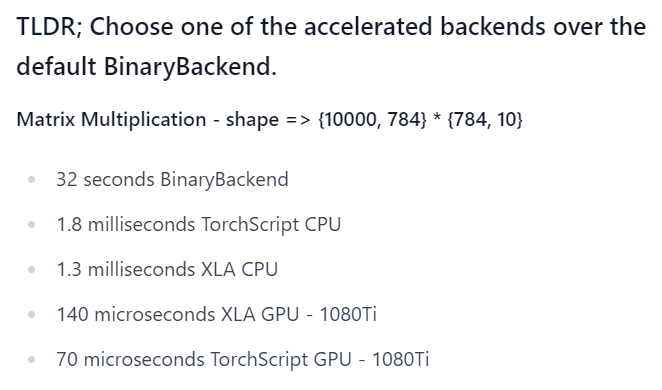
I’ve released a blog post where I introduce three Elixir notebooks that explore Elixir’s Nx backends, Along the Axon. Nx currently has 2 supported backends: PyTorch’s TorchScript and Tensorflow’s XLA. These notebooks are meant to correspond to the speed improvement portions of the 01_matmul Fast.ai notebook. In the TorchScript notebook, I demonstrate switching from the default BinaryBackend, to TorchScript on CPU, and then finally to TorchScript on GPU. I also have an XLA on GPU notebook and a XLA on CPU notebook. The speed seems in the range of Jeremy’s PyTorch notebook. If you try the notebooks and have any feedback that you don’t want to include here, I’m on the Fast.ai Discord also.