Lesson 12 official topic

This is a wiki post - feel free to edit to add links from the lesson or other useful info.

<<< Lesson 11Lesson 13 >>>

Lesson resources

Links from the lesson

Student notes

23 Likes

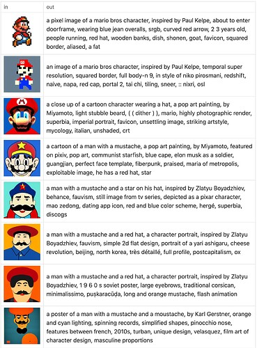
on the topic of CLIP Interrogator, I spent some time last week going back and forth through CLIP Interrogator and SD to see how an image evolves over time. :smile:

15 Likes

Does Einstein summation borrow anything from APL?

1 Like

If we pass in cuda.grid() for the numba function/kernel, how does it know the dimensions to create?

Would you recommend Numba over CuPy to do operations on the GPU?

1 Like
  • einsum is now a part of einops
2 Likes

A question about CLIP Interrogator: I have been looking into this idea since the weekend actually, and I noticed that CLIP has a image encoder. But this image encoder generates an embedding with 1024 floats, while the text encoder generates one with 768 (if I am not wrong).

What is this image encoder? Couldn´t we use it to train a nnet to learn to encode and decode from CLIP embeddings? A teacher strategy…

Einsum version of “dist” could be:

sorry - don't want to spoil!
8 Likes

@fredguth check this out: not that complicated :wink:

Thank you for doing everybody’s homework. :grinning:

1 Like

Soo sorry , posted before the question: you should resist to look at message history :wink:
But even more interesting will be to einsum-mize the weighted average too!

4 Likes

Best Calculus course ever for Deep Learning: Mathematics for Machine Learning: Multivariate Calculus

It focuses more on developing intuition, rather than calculation or proofs.

@radek has also shared about this recently.


Videos can be watched for free. And I urge everyone to at least try them.

6 Likes

If you just want to watch the videos directly on YouTube, the playlist is here: https://www.youtube.com/playlist?list=PLiiljHvN6z193BBzS0Ln8NnqQmzimTW23

2 Likes

Weights and biases has this amazing and intuitive course on math, linear algebra, stats and probability.
Hope you find this helpful :slight_smile:
Weights and Biases - Math youtube playlist

3 Likes

sorry, check what?

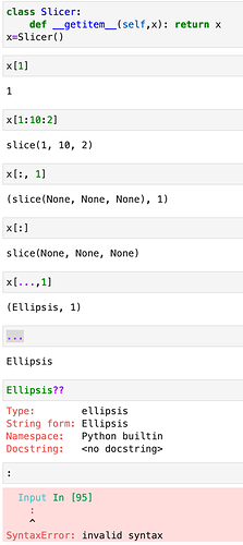
If anyone was wondering how the x[..., None] translate to Python objects, the ... means Elipsis that is a similar object to None. You can use it in typing and instead of pass when defining a function without the body. Here is the code if you want to play with it yourself.

6 Likes

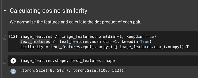
I think there are multiple sizes of clips and multiple trained models (on different data by different ppl). If you look at the original Clip repo and run the collab notebook, you will notice that they are presenting a version that outputs embeddings of size 512

link to clip colab and github repo:

DreamStudio recently got a “clip guidance” feature that It seems to be a way of using the newly trained clip model by laion with an already trained diffusion model. They do by a smart trick.

So clip is does not mean a specific model anymore :slight_smile:

4 Likes

Different CLIP models have different embedding sizes (512, 768 or 1024 are the options I think). Typically you need to use the right (text_encoder, image_encoder) pair - the embeddings from the text encoder of one CLIP model won’t map directly to those from the image encoder of another unless the models have the same embedding dimension and were trained in a way that kept them aligned.

As for your idea of a model to go directly from a CLIP image embedding back to an image in one shot: this is a hard task! It becomes like a very high-compression autoencoder. The closest I’ve seen to a working implementation is clip2latent which learns a mapping from CLIP embeddings (text or image) to styleGAN latents, allowing you to add text or image ‘prompting’ to any styleGAN model.

7 Likes

A few of us had a go at Jeremy today for explaining the Chain Rule by writing

\frac{dy}{dx} = \frac{dy}{du} \frac{du}{dx}

and “cancelling out” the du's — which isn’t kosher, because a derivative isn’t really a fraction! (It’s just the limit of a fraction.)

So what would be a kosher way of understanding the chain rule? Well, I think the way to think about it is to think of a derivative as “replacing” a curve by a linear function that is tangent to the curve at a given point: e.g. f(x) \approx \frac{df}{dx}(x_0)x + \text{some constant} for values of x close to x_0.

Now, what happens if we compose two linear functions? Let’s try it with f(x) = mx + c and g(x) = nx + d:

g(f(x)) = n(mx + c) + d = nmx + nc + d.

So what’s the slope of the composite function? It’s nm, which is the product of the slopes of the two component functions!

To bring everything full-circle, let’s say we want to compute \frac{dy}{dx} at some value x=x_0; and let’s say that u_0 is the value of u corresponding to x_0. Then we have

y \approx \frac{dy}{du}(u_0)u + c

for some constant c, and values of u close to u_0; and

u \approx \frac{du}{dx}(x_0)x + d

for some constant d, and values of x close to x_0. Composing the two, we have

y \approx \frac{dy}{du}(u_0)\left(\frac{du}{dx}(x_0)x + d\right) + c = \frac{dy}{du}(u_0)\frac{du}{dx}(x_0)x + \text{some stuff}.

Since this is true for any arbitrary value of x_0, and since u_0 is uniquely determined by x_0, we can drop both u_0 and x_0 from the above expression. Thus we see that the slope of y with respect to x — i.e. \frac{dy}{dx} — is nothing more than \frac{dy}{du} \frac{du\vphantom{y}}{dx}! No cancellation required.
6 Likes