Yeah it’s been bothering me too.
2 Likes
Thinking this would do:
learn,run = get_learn_run(nfs, data, lr=number|slice|callback_fn, ....)
Plus another wish-list, in fit print out the used hyperparams by default and have an option to turn off the printout (perhaps with a global defaults.fit_param_print = False). This would be so helpful at making sure she runs with the args she thinks she does. And it’ll help with calls for help - “why my setup is not training” as the report would include the actual used params.
2 Likes
I asked a question inaccurately.
I see it explained in lecture and in notebook.
I don’t understand why we can’t change order.
As i understand, if we will change order, first label every item in imagelist and then split, it will be same result in this case, when train / validation separated by folders.
But in case when we split by random, it possible situation when it might be missing rare classes in train or in validation sets.
And we want building universal process.
So i wonder if some reason process only train first and then validation (and may be test) with the same Processor, instead of full dataset.
Is it because of nlp or tabular data?
It won’t miss anything. Your model won’t be able to predict labels that are only in your validation set so doing it this way will throw an error when you have classes that are only present in your validation set, which is what you want to be warned this unwanted behavior is happening.
Of course it can happen! It is a random split: some rare classes might end in the valid set and your model will never learn from them.
In this case you have 3 options from my perspective :
- hope that your model could generalize well and fit the unseen data(but likely not with the unknown label),
- use the K-fold cross validation if the size of your data allows you that,
- make copies of the rare cases and add them to your training set.
Maybe these links about exponentially weighted averages, momentum, RMSprob, and Adam from the Andrew Ng DL course are helpful for others:
- Understanding Exponentially Weighted Averages
- Bias Correction of Exponentially Weighted Averages
- Gradient Descent With Momentum
- RMSProp
- Adam (Momentum + RMSprop)
- Link to the slides from the videos
This lesson was by far the most intense one! Keep up the great work! 
13 Likes
aren’t these mathematically equivalent ?
They are indeed identical: torch — PyTorch 2.4 documentation
p + (-lr / debias1) * grad_avg / ((sqr_avg/debias2).sqrt() + eps))

p + -lr * (grad_avg / debias1) / ((sqr_avg/debias2).sqrt() + eps))
Is there a pytorch guide that explains when to use this kind of do-many-things ops, as compared to doing it just the “normal” way, like in the expanded version above? I suppose the above way would be slower.
1 Like
Some questions that came up while going through the 09_optimizers.ipynb notebook:
For SGD with weight decay we use steppers = [weight_decay, sgd_step] so we run first weight_decay and then the output of it through sgd_step. However, in the notebook the full wd formula is shown as:
new_weight = weight - lr * weight.grad - lr * wd * weight.
Therefore, I wonder, if the sequential calculation is changing the weight to the “decayed weights”, which are then used for the sgd_step and we end up with something similar but not exactly what is outlined in the formula.
I tried to test the difference by combining
def weight_decay(p, lr, wd, **kwargs):
    p.data.mul_(1 - lr*wd)
    return p

def sgd_step(p, lr, **kwargs):
    p.data.add_(-lr, p.grad.data)
    return p
into a single (not really optimized) stepper
def sgd_weight_decay(p, lr, wd, **kwargs):
    sgd = -lr * p.grad.data
    wd = -lr * wd * p.data
    p.data.add_(sgd).add_(wd)
    return p
and run both 3x in the notebook with 10 epochs, but a real difference was not visible in the losses/accuracies.
1 Like
if we update with sgd first then wd (that is [sgd_step, weight_decay] ) then the result must be different, because we then use the sgd updated weights to calculate the wd term. However the difference is probably within the random variation of sgd
2 Likes
One of my favorite part of the fast.ai courses are that we are taught what are the latest state of the art methods.
I wonder for each new technique, does it just improve convergence, or does it improve the final result? Or both?
For example, should we expect a new optimizer to improve the final results? What about running batch norm?
Is it just a matter of reading the papers as well as trying things out?
Thanks
I had the same Idea but it didn’t work for me. When I run:
%time run.fit(2, learn)
after the weight initialization sometimes it works well but half of the time the loss either explodes or vanishes.
Did you attempted to train the model after the initialization? How did that work for you?
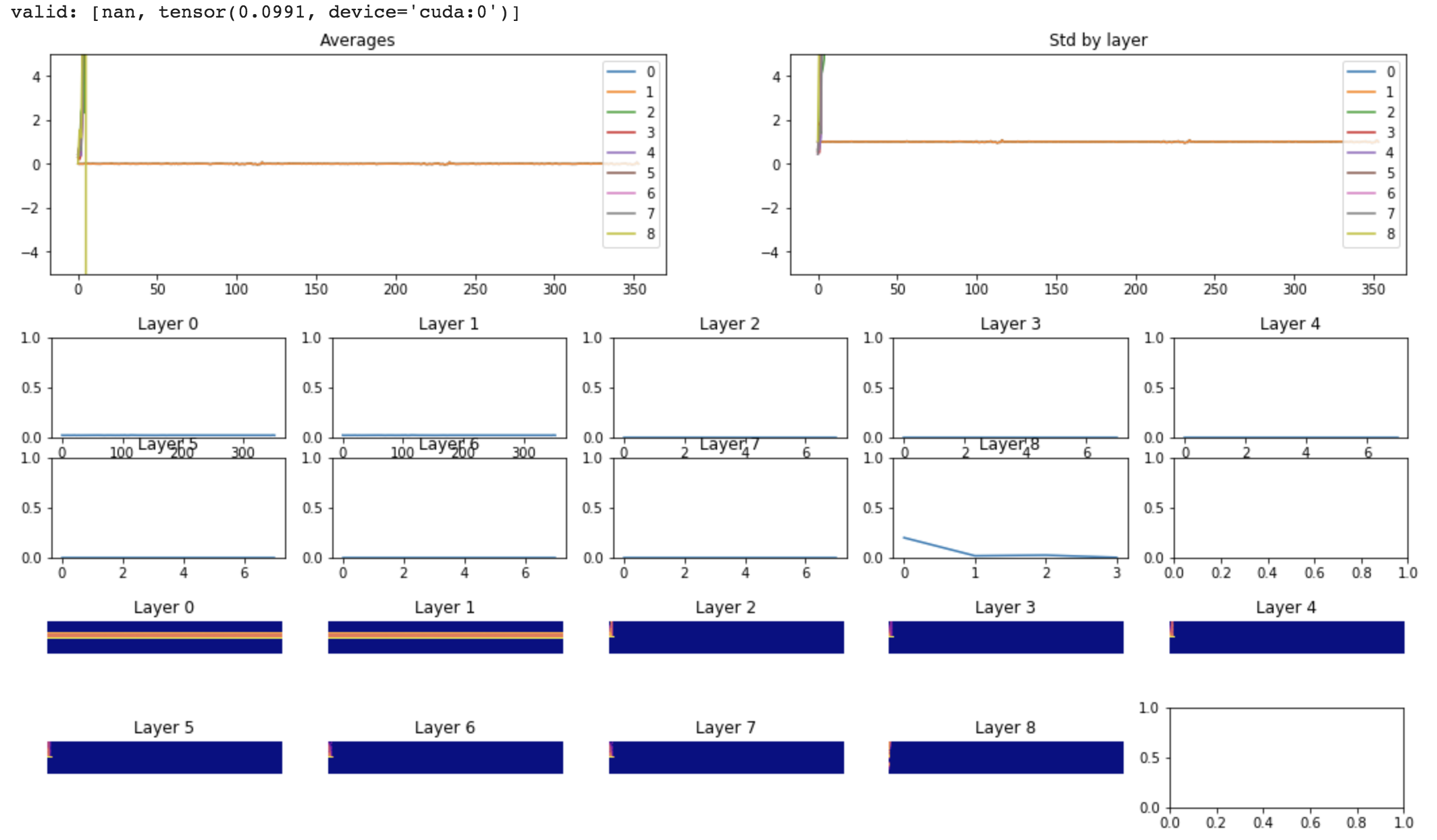
Bah! You’re right, @Kagan! It doesn’t train!
Indeed I only tested the stats and assumed the rest would just work! Thank you for checking that my suggestion was wrong!
I tried to re-normalize the stats part again, so std+bias+std, but no, that doesn’t work either.
Re-running lsuv_module twice destroyes training too!
for m in mods: print(lsuv_module(m, xb), lsuv_module(m, xb))
Anybody has an idea why? It looks like it’s very important that the bias is not zero-centered!
2 Likes
It was zeroed in their original pytorch impl anyway (github). In my experiments zero init was as good as fast.ai-style
Would it be possible to have a look at your full code/telemetry? Curious if we ran into the same thing
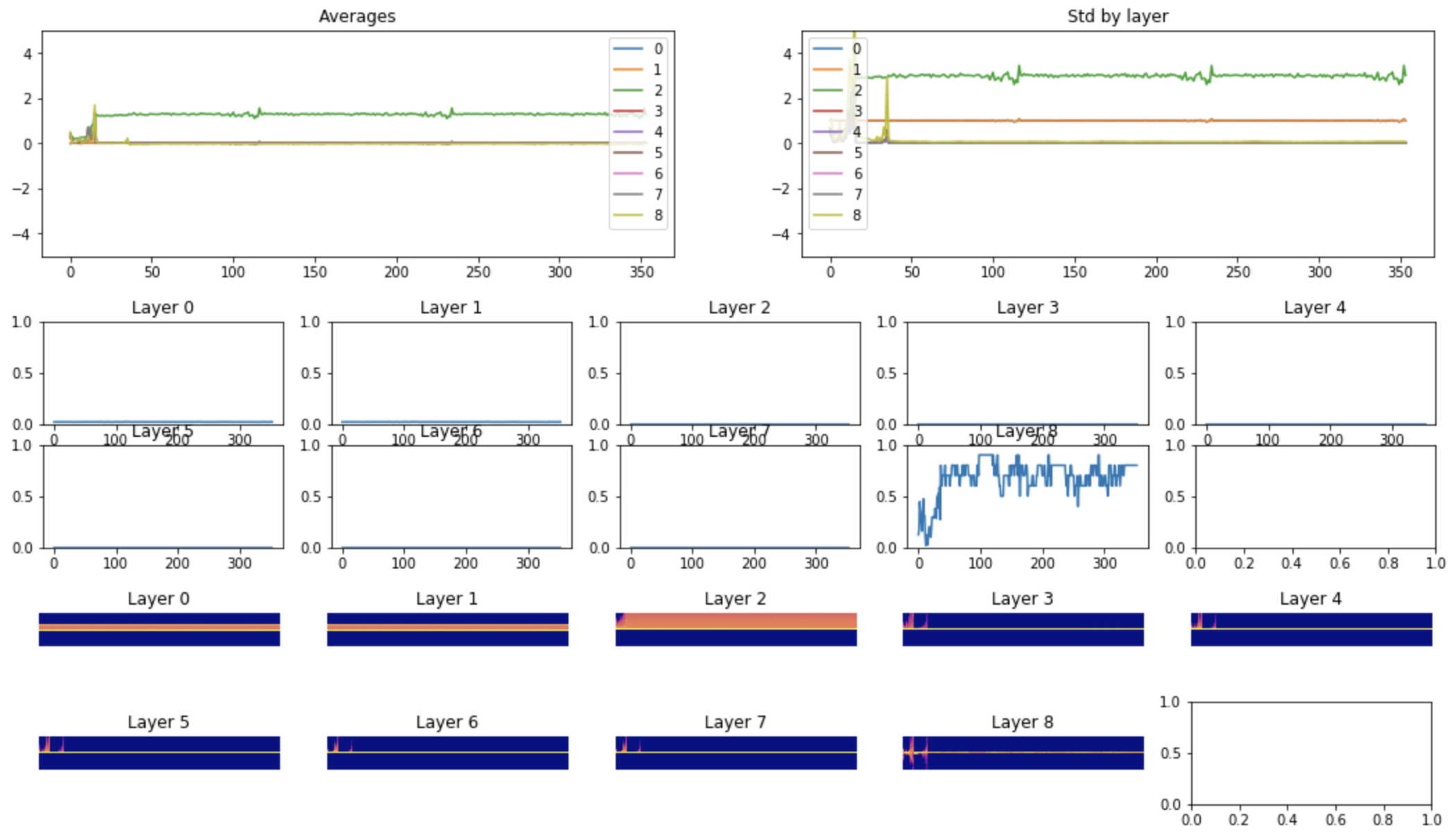
Had a similar symptom 1/2 of the trainings
Fixed by reducing LR from 1 to 0.4, here’s how that looked on telemetry
It’s just 07a_lsuv.ipynb as is.
Here is another variant I tried, attempting to balance the adjustments, while having std=1, mean=0 post-lsuv_module:
def lsuv_module(m, xb):
    h = Hook(m, append_stat)

    while mdl(xb) is not None and (abs(mean) > 1e-3 or abs(std-1) > 1e-3):
        mean,std = h.mean,h.std
        if abs(mean)  > 1e-3: m.bias -= mean
        if abs(std-1) > 1e-3: m.weight.data /= std

    h.remove()
    return h.mean,h.std
(note: it recalculates mean/std twice, but I didn’t bother refactoring, since it’s just a proof of concept.)
it works better (i.e. trains), but still getting nans every so often. This is with the default lr=0.6 of that nb.
But, of course, the original nb gets nans too every so often, so that learning rate is just too high.
With a lower lr=0.1the original reversed order std+bias approach trains just fine too.
Here is a refactored “balanced” version:
def lsuv_module(m, xb):
    h = Hook(m, append_stat)

    while mdl(xb) is not None:
        mean,std = h.mean, h.std
        if abs(mean) > 1e-3 or abs(std-1) > 1e-3 :
            m.bias -= mean
            m.weight.data.div_(std)
        else: break

    h.remove()
    return h.mean,h.std
Perhaps self.sub in GeneralReLU needs to be a parameter and then the init will only affect the initial setting and then let the network tune it up.
2 Likes
Thank you for checking this out. it’s good to know that we can mitigate the exploitation/vanishing by reducing the learning rate.
It’s still kind off weird that this happening though, I’d expect lsuv std+bais to perform the best since it have the “perfect statistics”.
I thought that it might be related to the distribution of the weights after the initialization (having 0 mean, 11 std, but being skewed) so I plot a histogram after the initialization
for m in mods: plt.figure(); plt.hist(m.weight.view(-1).detach().cpu(), bins = 20)
but it looks pretty much the same when model trains normally and when it goes to NaN
I played some more with 07a_lsuv nb. Here are some observations/notes:
-
The
subargument shouldn’t be configurable as it gets reset to a value relative to the batch’s mean regardless of its initial value. (Unless, it’s meant to be used by some other way w/o lsuv, but it’d be very difficult to manually choose, as it varies from layer to layer with lsuv.)To prove that it doesn’t need to be configurable, fix the seed and re-run the nb once with
subset to 0 and then to 50, adding its value to the return list - afterlsuv_moduleis run -m.relu.subends up being exactly the same value, regardless of its initial value.
class ConvLayer(nn.Module):
    def __init__(self, ni, nf, ks=3, stride=2, sub=50., **kwargs):
                                               ^^^^^^^
    [...]

def lsuv_module(m, xb):
    [...]
    return m.relu.sub, h.mean, h.std
           ^^^^^^^^^^
-
making
suba parameter didn’t lead to improvements, but made things worse in my experiments. the value ofsubseems to be a very sensitive one. -
this implementation of lsuv doesn’t check whether variance is tiny (no eps) or undefined (small bs w/ no variance) before dividing by it - it tests with bs=512 which won’t have any of these issues, which is far from a general case.
using bs=2 requires a much much lower lr
-
While experimenting I used a random reproducible seed, so it was helpful to analyse closer the cases where the network wasn’t training (so that I could turn different parts on/off). Most of the time lsuv seemed to be the culprit - so it is helpful in general, but also leads to
nans at times at the lr used in the nb.
Also note that the original LSUV doesn’t tweak the mean, only the std. But w/o the mean tweak in the lesson nb, things don’t perform as well. So this is a bonus. And the nb version doesn’t implement the optional orthonormal init.
5 Likes
Hi,
According to 10_augmentation.ipynb, using numpy is supposed to result in faster tensor creation, but that’s clearly not happening for me. Not sure what could be going on; I repeated this test with 2 more images:
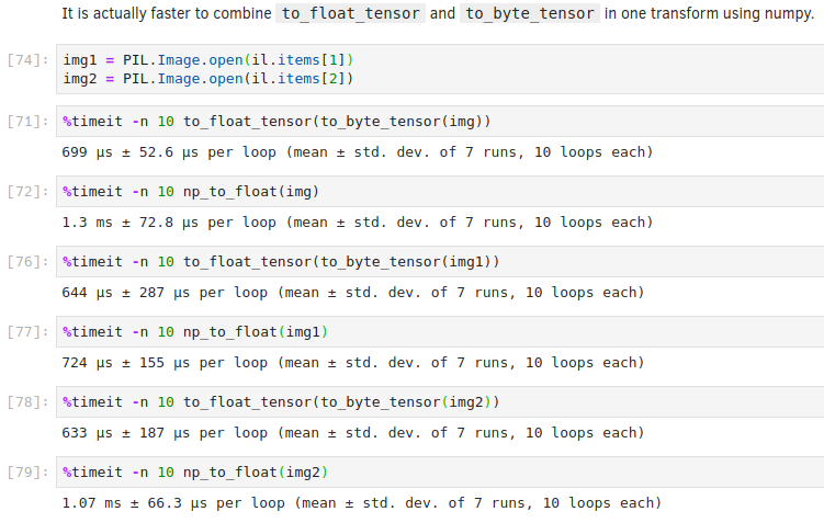
That’s interesting. I guess it might depend on the Pillow, pytorch, and numpy versions…
Just a quick really pedantic domain specific comment on RandomResizeCrop which from lesson sounds like fastai is looking to replace with very smart perspective “warp” transform.
Jeremy made comments that objects are never wider or thinner in the real world and that RandomResizeCrop is perhaps trying to account for changes in perspective.
Knowing the behavior of camera lenses RandomResizeCrop still serves a purpose. For example, some lenses will result in faces in portraits (i.e. objects) appear wider while others will make it appear thinner.
See site as first google search reference on this. https://mcpactions.com/2014/05/19/perfect-portrait-lens/
In short. I think a combination of both could be useful.