From my understanding of lens distortion that’s not quite true - they don’t squish an entire picture just horizontally or vertically. Or at least not enough to make the massive squishing of imagenet transforms sensible.
in the code of this lesson 11, is there any dropout being applied by pytorch undernearth during training? or does it have to be explicitely called for? thank you 
Here is something I’m confused about:
At around 01:22:00 in the lesson, talking about momentum, Jeremy says that if you have 10 million activations, you need to store 10 million floats. Did he mean weights instead of activations? Because a bit before that he called them parameters (which, as I understand, are the same as weights), and a bit before that he also called the activations (which are very different).
Thanks.
Probably I have missed something, but I do not understand why we choose kernel size 3 insted of 5 for the first layer? If that is something proven by research, can you explain me why Jeremy has choosen the number of channels for the first layer to be c_inx3x3. I did not undestant that part neither 
Actually I think it is in this other „bag of tricks“ paper, somewhat inflationary use of the term ;-):
Page 5:
The observation is that the computational cost of a convolution is quadratic to the kernel width or height. A 7 × 7 convolution is 5.4 times more expensive than a 3 × 3 convolution. So this tweak replacing the 7 × 7 convolution in the input stem with three conservative 3 × 3 convolutions […]
1 Like
Oops I copied from Google without checking - deleted my reply so others won’t be confused.
1 Like
Dear @jeremy, thank you sooo much for that moment: 
" we show that L2 reg has no regularisation effect…WHAT??? … "
… "
" you know how I keep mentioning how none of us know what they are doing… that should make you feel better about ‘can I contribute to DL’ …? "
It does. I love your way of teaching, encouraging us, knocking down the barriers of entry to deep learning and gifting us all these tips and tools, but THAT WAS BY FAR THE BEST, MOST ENCOURAGING MOMENT so far for me. I was just thinking “my head is about to explode with all this info, I need a walk, fresh air” and boom you dropped the mic.
Thanks again and please keep in coming,
Lamine Gaye
PS: my 1st post on the forums… I just had to say this
2 Likes
At around 28:00, Jeremy talks about get_files(), and how fast it is. I was intrigued, and decided to try to recreate it locally and experiment. I wanted to start off with a naive version and see what sort of speed ups I could achieve:
def get_fnames(train=False):
    path = Path('/Users/daniel/.fastai/data/imagenette-160')
    if train:
        path = path/'train'
    else:
        path = path/'val'

    fnames = []
    for _dir in path.ls():
        for fname in _dir.ls():
            fnames.append(fname)

    return fnames
>>> fnames = get_fnames(train=True)
>>> len(fnames)
12894
>>> timeit -n 10 get_fnames(train=True)
34.9 ms ± 1.16 ms per loop (mean ± std. dev. of 7 runs, 10 loops each)
>>> fnames[:3]
[PosixPath('/Users/daniel/.fastai/data/imagenette-160/train/n03394916/n03394916_58454.JPEG'),
 PosixPath('/Users/daniel/.fastai/data/imagenette-160/train/n03394916/n03394916_32588.JPEG'),
 PosixPath('/Users/daniel/.fastai/data/imagenette-160/train/n03394916/n03394916_32422.JPEG')]
In the video, he shows ~70ms runtime, whereas I’m getting ~35, about twice as fast. This suggests I’ve misunderstood the task at hand or something … can anyone shed any light on what’s going on? Are we in fact doing the same thing? Why does my timing show a faster speed?
Don’t see this mentioned here in Lesson 11 thread, so adding a link here.
If you get the following errors when running 08_data_block.ipynb
-
cos_1cycle_annealnot defined -
Runnerdoes not havein_train
Link to forum thread discussing this and the solution - thanks to @exynos7 for spending the time to solve for all of us.
1 Like
A minor tweak that fixes the LSUV algorithm normalization
Note added: I found after writing this post that @stas independently discovered this a while ago
At the end of the 07a_lsuv.ipynb notebook, the means and stds of each layer are shown after the application of the LSUV algorithm, and we see that the means are not near zero.
There is a comment in the notebook: “Note that the mean doesn’t exactly stay at 0. since we change the standard deviation after by scaling the weight.”
However, if in the lsuv_module you first scale the standard deviation, then correct the mean, the problem with the not-near-zero means is solved. This involves switching the order of two lines of code as follows:
Original version:
while mdl(xb) is not None and abs(h.std-1) > 1e-3: m.weight.data /= h.std
while mdl(xb) is not None and abs(h.mean) > 1e-3: m.bias -= h.mean
Modified version:
while mdl(xb) is not None and abs(h.mean) > 1e-3: m.bias -= h.mean
while mdl(xb) is not None and abs(h.std-1) > 1e-3: m.weight.data /= h.std
In the next cell, we execute the lsuv initialization on all layers and print the means and standard deviations of the weights:
for m in mods: print(lsuv_module(m, xb))
Here is the output with the modified code:
(-2.3492136236313854e-08, 0.9999998807907104)
(2.5848951867857295e-09, 1.0)
(-1.7811544239521027e-08, 0.9999998807907104)
(9.778887033462524e-09, 0.9999999403953552)
(-1.30385160446167e-08, 1.0000001192092896)
The normalization is now perfect (i.e., within the specified precision) in both mean and standard deviation. However, fixing the mean to be near zero did not improve model accuracy.
1 Like
In the paper “All you need is a good init” the authors say that their Algorithm 1 is intended to follow a certain orthonormal initialization procedure: “We thus extend the orthonormal initialization Saxe et al. (2014) to an iterative procedure, described in Algorithm 1. Saxe et al. (2014) could be implemented in two steps. First, fill the weights with Gaussian noise with unit variance. Second, decompose them to orthonormal basis with QR or SVD decomposition and replace weights with one of the components.”
Question @Sylvain, @stas or anyone else who knows: why did Fastai omit the Saxe et al. (2014) orthonormal initialization procedure?
2 Likes
The following block of code in the Jit version section at the end of the 10_augmentation notebook
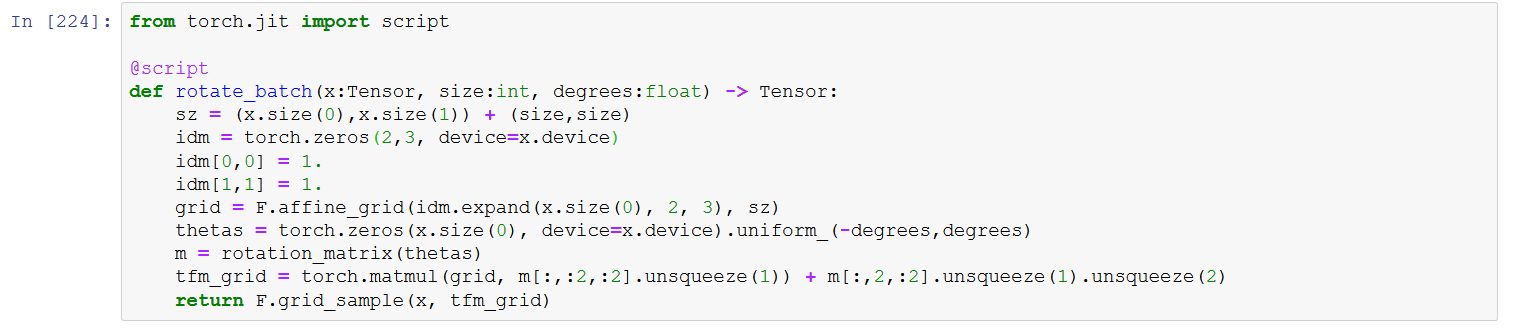
throws a RuntimeError (see below).
I am running Windows 10 64-bit. Has anyone seen this problem?
RuntimeError Traceback (most recent call last)
in
2
3 @script
----> 4 def rotate_batch(x:Tensor, size:int, degrees:float) -> Tensor:
5 sz = (x.size(0),x.size(1)) + (size,size)
6 idm = torch.zeros(2,3, device=x.device)
~\Anaconda3\envs\fastai\lib\site-packages\torch\jit_init_.py in script(obj, optimize, _frames_up, _rcb)
1179 return obj
1180 else:
-> 1181 return _compile_function(fn=obj, qualified_name=qualified_name, _frames_up=_frames_up + 1, _rcb=_rcb)
1182
1183
~\Anaconda3\envs\fastai\lib\site-packages\torch\jit_init_.py in _compile_function(fn, qualified_name, _frames_up, _rcb)
1075 return result
1076 return stack_rcb(name)
-> 1077 script_fn = torch._C._jit_script_compile(qualified_name, ast, _rcb, get_default_args(fn))
1078 # Forward docstrings
1079 script_fn.doc = fn.doc
~\Anaconda3\envs\fastai\lib\site-packages\torch\jit_init_.py in _try_compile_fn(fn, loc)
1008 rcb = _jit_internal.createResolutionCallbackFromClosure(fn)
1009 qualified_name = _qualified_name(fn)
-> 1010 return _compile_function(fn, qualified_name=qualified_name, _frames_up=1, _rcb=rcb)
1011
1012
~\Anaconda3\envs\fastai\lib\site-packages\torch\jit_init_.py in _compile_function(fn, qualified_name, _frames_up, _rcb)
1075 return result
1076 return stack_rcb(name)
-> 1077 script_fn = torch._C._jit_script_compile(qualified_name, ast, _rcb, get_default_args(fn))
1078 # Forward docstrings
1079 script_fn.doc = fn.doc
RuntimeError:
Arguments for call are not valid.
The following operator variants are available:
aten::div(Tensor self, Tensor other, *, Tensor(a) out) -> (Tensor(a)):
Expected a value of type ‘Tensor’ for argument ‘self’ but instead found type ‘float’.
aten::div(Tensor self, Tensor other) -> (Tensor):
Expected a value of type ‘Tensor’ for argument ‘self’ but instead found type ‘float’.
aten::div(Tensor self, Scalar other) -> (Tensor):
Expected a value of type ‘Tensor’ for argument ‘self’ but instead found type ‘float’.
aten::div(int a, int b) -> (float):
Expected a value of type ‘int’ for argument ‘a’ but instead found type ‘float’.
aten::div(float a, float b) -> (float):
Expected a value of type ‘float’ for argument ‘b’ but instead found type ‘int’.
div(float a, Tensor b) -> (Tensor):
Expected a value of type ‘Tensor’ for argument ‘b’ but instead found type ‘int’.
div(int a, Tensor b) -> (Tensor):
Expected a value of type ‘int’ for argument ‘a’ but instead found type ‘float’.
The original call is:
at :2:17
def rotation_matrix(thetas):
thetas.mul_(math.pi/180)
~~~~~~~~~~~ <— HERE
rows = [stack([thetas.cos(), thetas.sin(), torch.zeros_like(thetas)], dim=1),
stack([-thetas.sin(), thetas.cos(), torch.zeros_like(thetas)], dim=1),
stack([torch.zeros_like(thetas), torch.zeros_like(thetas), torch.ones_like(thetas)], dim=1)]
return stack(rows, dim=1)
‘rotation_matrix’ is being compiled since it was called from ‘rotate_batch’
at :11:5
@script
def rotate_batch(x:Tensor, size:int, degrees:float) -> Tensor:
sz = (x.size(0),x.size(1)) + (size,size)
idm = torch.zeros(2,3, device=x.device)
idm[0,0] = 1.
idm[1,1] = 1.
grid = F.affine_grid(idm.expand(x.size(0), 2, 3), sz)
thetas = torch.zeros(x.size(0), device=x.device).uniform_(-degrees,degrees)
m = rotation_matrix(thetas)
~~~~~~~~~~~~~~~~~~~~~~~~~~ <— HERE
tfm_grid = torch.matmul(grid, m[:,:2,:2].unsqueeze(1)) + m[:,2,:2].unsqueeze(1).unsqueeze(2)
return F.grid_sample(x, tfm_grid)
1 Like
I totally love the idea of performing image data augmentation on the GPU. After all, GPUs were originally designed to speed up the calculations required to display environments from different perspectives, e.g. in computer games.
Not sure if someone already mentioned this but for LSUV if you want to get your means even closer to zero, just do the variance normalization before the mean normalization, then do the variance normalization again. The second time will not change as much:
lesson:
def lsuv_module(m, xb):
    h = Hook(m, append_stat)

    while mdl(xb) is not None and abs(h.mean)  > 1e-3: m.bias -= h.mean
    while mdl(xb) is not None and abs(h.std-1) > 1e-3: m.weight.data /= h.std

    h.remove()
    return h.mean,h.std
results in:
(0.17517215013504028, 1.0)
(0.11678619682788849, 1.0)
(0.16046930849552155, 0.9999999403953552)
(0.19877631962299347, 1.0)
(0.30298691987991333, 0.9999999403953552)
my tiny fix:
def lsuv_module(m, xb):
    h = Hook(m, append_stat)

    while mdl(xb) is not None and abs(h.std-1) > 1e-3: m.weight.data /= h.std
    while mdl(xb) is not None and abs(h.mean)  > 1e-3: m.bias -= h.mean
    while mdl(xb) is not None and abs(h.std-1) > 1e-3: m.weight.data /= h.std

    h.remove()
    return h.mean,h.std
results in:
(-5.817306828248547e-06, 1.0)
(-2.4605162707302952e-06, 1.0)
(1.9352883100509644e-06, 1.0)
(6.183981895446777e-07, 1.0)
(1.0989606380462646e-06, 1.0)
You can of course play that game to infinity but even adding that one line got my means to basically zero from 0.1-0.3 absolute before.
Yes, I’d noted this recently
I found that I didn’t need to iterate the std normalization as in your second code block; the means were reduced to ~1.e-8 after switching the while statements.
Subsequently, I found that @stas had already made the same discovery
But @Kagan found that the idea doesn’t work, and @stas verified this.
Also @SteveR had similar idea , which @stas had also considered.
2 Likes
Cool, thanks for pointing me to the discussions, @jcatanza!
1 Like
The implementation of SGD with momentum in the lesson notebook updates the grad_avg like this:
state['grad_avg'].mul_(mom).add_(p.grad.data)
Shouldn’t it be updating it like this instead:
state['grad_avg'].mul_(mom).add_(1-mom, p.grad.data)
i.e. taking 0.9 part of the previous and (1-0.9 = 0.1) part of the current gradient (if mom=0.9)?
In Lesson 5, when momentum was explained using Excel, that’s what we did: see https://youtu.be/CJKnDu2dxOE?t=6569
I do see that further down in the notebook, for Adam, we do account for this, and also add debiasing.
Why does it happens when I run this cell in jupyter notebook.
The code is copied from the source code from github…
Could anybody help me about this?
I thought I wrote the code accurately…

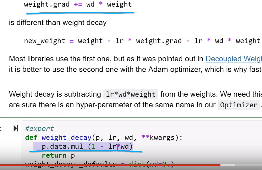
In Decoupled Weight Regularization by Ilya Loshchilov and Frank Hutter, they propose to use w' = w - lr * [adam(grad) + wd * w], but that isn’t what the generic optimizer with steppers=[adam_step,weight_decay] is doing.
The steppers are doing
tmp = w - lr * adam(grad)
w' = tmp * lr * (1-wd)
or
w' = w * lr * (1-wd) - lr^2 * adam(grad) * (1-wd)
which appears different from what Ilya and Frank intended. In particular, the lr^2 * adam(grad) term quickly vanishes as lr decreases and may cause numerical stability issues and zero out some adam updates.
Experiment:
I ran some simple experiments with the 09_optimizers notebook, using the
learn,run = get_learn_run(nfs, data, 0.001, conv_layer, cbs=cbfs, opt_func=adam_opt())
run.fit(3, learn)
cells with some tweaks:
- I noticed that repeated calls to the same cells had high variance, so I set the seeds
def fix_seeds(n): random.seed(n); torch.manual_seed(n)and ran each experiment for 3 seeds (7, 42, 10914). (There is still some nondeterminism between runs with those seeds fixed, but the variance is dramatically reduced). - I increased the number of epochs from 3->10, since the impact of weight decay increases as we increase the risk of overfitting.
Results:
- For the baseline with
wd=0, I observed accuracies of 0.5715, 0.5929, 0.5710 (mean=0.5785). code - With
steppers=[adam_step,weight_decay]andwd=1e-2, I observed accuracies of 0.5768, 0.6056, 0.5832 (mean=0.5885) code - With combined steppers and
wd=1e-2, I observed accuracies of 0.5750, 0.6132, 0.5857 (mean=0.5913) code
So based on the above calculations and experiments, I don’t think we can cleanly split the adam and weight decay steps into separate functions. A combined adam + weight decay step can lead to higher validation accuracy.