Lesson 1 In-Class Discussion ✅

@gluttony47 I found a solution using a cobination of threads.

I used this thread to create a conda environemnt: Fastai v0.7 install issues thread

I then used this thread to actually run the notebooks. You have to activate the environment, then start a jupyter notebook port, then start another ssh connection in another bash and connect there: How to setup fastai v0.7 on gcp instance that is setup for 2019's Part 1

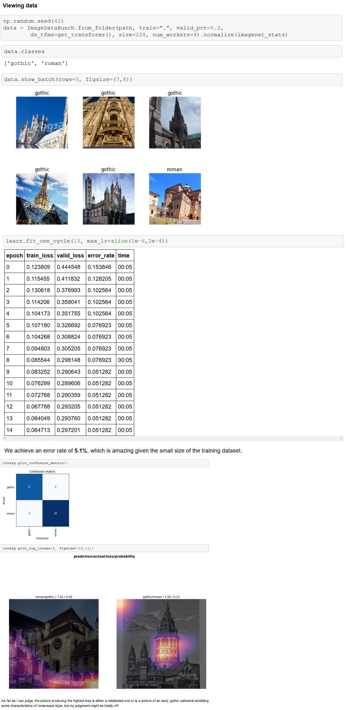
Based on what is taught in Lesson 1, I trained a resnet50 model to classify pictures of romanesque cathedrals vs. gothic cathedrals. I achieved an error rate of 5.1%. My notebook along with the textfiles containing the urls of the images I used for training and validation can be found here: https://github.com/g-vk/fastai-course-v3

Here is a preview of the notebook:

2 Likes

Notes of Lesson 1 with some of my additions and clarifications. Hope some will find it helpful. Feel free to leave any comments.

1 Like

Great job @gvolovskiy…I have a doubt…following the notebook lesson, I understood that the learning rate must be found before the unfreeze step. Something like that:
learn.load(‘stage-1’)
learn.lr_find()
learn.recorder.plot()
learn.unfreeze()
Pls let me know!

Before unfeezing, the set of trainable parameters is the same as when training the head of the model. Since after loading the stage-1 weights the weights of the head of the model are already trained, there is no need to train them again and hence also to look for a good learning rate. It is only after we enlarge the set of trainable parameters by invoking learn.unfreeze() that looking for a suitable learning rate becomes necessary.
I hope my explanaion was helpful for you.

1 Like

Thanks for the explanation!

**Edit:
I was not aware that the heat map are by design set to true in the plot_top_losses function.

Hi all

I’m having an issue when I try to show the top losses, the images comes out distorted
what can be the issue here ?

Thank you for sharing - it really helped us! :slight_smile:

1 Like

Glad to hear. Thanks

What do you mean by distorted? Your screenshot looks fine to me. Did you try a bigger figure size? figsize=(12,12)

For what it’s worth, you might consider switching from GCP to Salamander simply because Salamander appears to be operated by the same people who operate FastAI. Either that or it’s very closely integrated; point being that setting up FastAI with Salamander is quite easy.

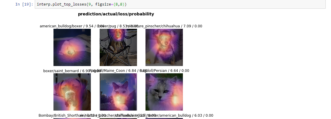
Are you referring to the colored blobs that appear on each image? Those are called heatmaps and they are supposed to show you which portion of the image the neural net is “most interested” in, so to speak.

From the Fast.AI documentation on plot_top_losses():

plot_top_losses [source]

plot_top_losses ( k , largest = True , figsize = (12, 12) , heatmap : bool = None , heatmap_thresh : int = 16 , return_fig : bool = None ) → Optional [ Figure ]

When heatmap is True (by default it’s True) , Grad-CAM heatmaps (http://openaccess.thecvf.com/content_ICCV_2017/papers/Selvaraju_Grad-CAM_Visual_Explanations_ICCV_2017_paper.pdf) are overlaid on each image.


Hope that helps you understand the heatmap “distortions”.

Got it, thanks a lot for the clarification

I guess I mistook the heat maps as something wrong with the pictures, thanks to @knakamura13 for pointing that out to me

1 Like

I just finished watching the Lesson 1 and I think I’ve understood the concepts well. Also, got the same working on my notebook. My question is - If I want to take one image specifically of my own and test what the output of the classifier would be, how do I go about it?

I’d go watch lesson 2, Jeremy covers exactly that! :slight_smile:

Hello @gluttony47 I’m late to your post. I just wanted to say that I also picked GCP and it is a difficult thing to get installed imo. You have to keep playing with it. It took me a few days to get it to work. I was all over the forums & the GCP help pages too.

Great! Thanks

Hi everyone,

I hope I did not miss the answer to the following question somewhere in here:

Running the lesson in Google Colab multiple times (with resetting of the runtimes in between) I get different error rates in cell 16.

Now seeing that in cell 10 a seed is being set, I do not quite understand where the degree of randomness originates.

Can someone enlighten me on this please?

Thanks.

1 Like

I’m not sure if I can answer your question, but could you provide examples? How drastically are your error rates fluctuating?