Interpreting ActivationStats.color_dim graphs and fixing bad layers

I am having problems with my model and I am trying to solve where exactly problems are occurring…

I started using ActivationStats.color_dim graphs to try to find where might be my problem… But then I am left trying to interpret the graphs to try to fix the underlying problems. I have read the original post about the graphs which was quite useful for interpretation.

But now I want to fix the layers where problems are occurring. For example here are the layers of my network:

There are a several Linear layers which seems to have a concerning graph, for example:

image

But then I have a BatchNorm right after… So I guess this brings back the values to a normal range.

My question is what can I do to make those layers train more gracefully?

For anyone interested, I made a custom code snippet to plot all ActivationStats.color_dim graph for all layers in the model for anyone that could find this interesting (google didn’t have much results on how to use ActivationStats):

stats = ActivationStats(with_hist=True)
learner = Learner(dls, model, cbs=[stats])

#... fit here...

layers = [m for m in flatten_model(model) if has_params(m)]

for i, layer in enumerate(layers):
    fig, ax = plt.subplots(figsize=(16, 32))
    ax.set_title(layer)
    stats.color_dim(i, ax=ax)
4 Likes

I usually try to minimize @ people, but if the original author @ste has any advise that could be useful for other people, it would be awesome!

For example here is a simple TabularModel that seems to have a healthy trainning:

1 Like

My first guess would be are you using drop out? That may help some (also using it on my tabular model now, so cool!)

I’m assuming that your training a regression model according to the shape of the last layer and the number of outputs (=1), right?

The second question is why you don’t train the bias term on the last layer on the first model? …Pretty sure that the wavy behavior of the last layer is due to that :wink:

Btw if you want your training to be more “gentle” you can work on:

  • initialization (IE: All you need is a good init)
  • LR (ie: reducing it and/or increasing epochs - I’m assuming you’re training with cycles)
  • dropout as @muellerzr said or other regularization techniques like WD or L2 (maybe you’ll be able to figure out a way to do tabular data augmentation on your domain :wink: ).
  • try different activation function like Jeremy did on the lesson with LeakyRelu or SELU.
3 Likes

If I had to guess, this is the first layer after the embeddings from a tabular model (hence why the output is 200). Those do not have a bias :slight_smile: (Also I may go play around with LeakyRelu, SELU, and Mish now :wink: )

Interestingly enough, the implementations seem to differ ever so slightly (and possibly in a way that needs debugging). Let me explain. So if I take a look at a tabular model in the v1 version, I can look at the embeddings like so:


(the first 6 layers are my embeddings). We begin to see a peak there.

But in the v2 version I get something similar to what @etremblay shows, with the mildly blank picture minus a pixel on the bottom. I won’t @ Jeremy yet unless we can’t figure out what may be happening, but just realizing this bug :slight_smile:

Edit: another interesting observation, take for example these tabular embeddings:

This is the same variable twice (in L0 and L1). What in the world do I make of this? The larger the peak the more it’s utilized? :slight_smile:

4 Likes

I was talking about the last “tile” of the two charts:

  • First chart: Linear (in:60, out:1, bias: False)
  • Second chart: Linear (in:50, out:1, bias: True)

Isn’t that the last layer?

I see what you mean now! Yes :slight_smile: (I think?)

Thanks for the response! Sorry in advance for the wall of text below. If this is too much, feel free to enjoy your week-end :).

  • I will definitely try changing the bias term!
  • For the initialization, I thought this was handled by fastai by default, but maybe I am wrong!
  • lr_find is suggesting rather larger learning rates, I am using 1e-2 right now and wd=.4
  • The following code shows how much dropout I used for the TabularModel.
  • Excellent I will play around with activation functions too!

Here is the code for my model for the purpose of the discussion. It deals with hierarchical tabular data. So I mainly use TabularModel.

I have a questionnaire (parent), multiple questions per questionnaire (children). I want to predict the score of the questionnaire next time it gets answered. I pass in the questionnaire tabular info and I pass a collection of questions. Both as a collection of categorical and continuous variables.

The layer self.questions is simply a TabularModel that predict the score of the next question in a questionnaire, but it also returns returns the activations of the last layer of size 50 in the TabularModel. I pre-trained this model before because I thought I could use transfer learning by freezing it and fine tuning it later…

The result of size 50 from the pre-trained network is sum-ed together (this is basically the idea behind Deep Sets since questions order is not important). I concat this vector with the result from the TabularModel self.results and pass it in the head of the network that predicts the final score for the questionnaire. I am thinking of replacing the Deep Sets part with an Attention layer…

class ParentChildModel(Module):
    def __init__(self, questions):
        self.results = TabularModel(results_emb_szs, len(results_cont_names), 10, [200, 50], ps=[0.01, .1], embed_p=0.04, bn_final=False)
        self.questions = questions
        
        self.head = nn.Sequential(*[LinBnDrop(60, 1, p=0.), SigmoidRange(*[-1, 101])])

    def forward(self, data, children):
        parent_cat, parent_cont = data[0], data[1]
        results = self.results(parent_cat, parent_cont)
        
        questionScores = []
        batchQuestionMid = []
        for children_cat, children_cont, length in children:
            result, mid = self.questions(children_cat, children_cont)
            result = result.squeeze()
            batchQuestionMid += [mid.sum(axis=0)]
            questionScores += [F.pad(result, pad=(0,1000-len(result)), mode='constant', value=0)]
        
        batchQuestionMid = torch.stack(batchQuestionMid)
        concat = torch.cat([results, batchQuestionMid], axis=1)
        results = self.head(concat)
        
        questionScores = torch.stack(questionScores, dim=0)
        return results, questionScores

The network tries to predict both the scores of the questionnaire at the parent level, but also each individual question in it.

The loss function looks like this. It combines the loss for the questionnaire score and the question scores. Each questionnaire can have a variable number of question, so I have to account for that.

def combined_loss(output, target, question_target, question_lens):
    result_output, question_output = output

    res_pred, res_targets = [], []
    for i, x in enumerate(question_target):
        l = question_lens[i].item()
        res_pred += [question_output[i][:l]]
        res_targets += [x[:l]]
        
    question_output = torch.cat(res_pred).flatten()
    question_target = torch.cat(res_targets).flatten()
    
    return torch.mean((result_output - target)**2) + torch.mean((question_output - question_target)**2)
2 Likes

Thank you for sharing this Interesting approach! I’ll take for sure a look to the paper.

MODEL INSIGHTS
So you’re running two tabular model (Parent and Result): that’s the reason why in the sequence of charts you’ve sent there are two separated groups of “Embedding Layers”, one for each tabular model.

Following your forward pass and comparing it to the tiles i can see three main groups

  • P: Parent tabular model (27 tiles)
  • R: Result tabular model (25 tiles)
  • H: The final head (2 tiles)

The tabular models are made by stacking together all the embedding that came from CATEGORICAL variables and the result of a linear layer applied to the CONTINUOS ones. This stacked tensor is then passed trough the TABULAR HEAD (last two layer of the group).


See the “Rossmann paper” for details: Entity Embeddings of Categorical Variables

The forward pass can be thought as:

(results, questionScore) = forward( parentData, childrenData )

Where parentData and childrenData are tuple made of (categorical,continous) = (cat,cont) data.

At the beginning of forward pass the Parent model is run; then the result of P pass is somehow concat with the result of R pass applied to all childrenData. Eventually this concat tensor is feed to the head of the model and crunched to produce a single dimensional output (The last layer has out size = 1).

TRAINING INSIGHTS
So looking at the charts, it seems that P has more “influence” than R on the final output. I say that because, despite there is no bias term learning on the last layer, it seems that the fluctuations on P affect the output more than the variations on R.

According to my experience, “balancing multiple forces” during training is a pretty complicated thing that usually doesn’t come out of the box, depends on your data and almost always involve a mixture of hack on the forward pass and the loss function (as your are doing :wink: )… So good luck!

I’m pretty curious to see how your tiles chart changes after changing some hyperparameters :wink:

5 Likes

Thanks for your reply! What app are you using to make those drawing? This really helps with understanding.

I think the main problem that I have is the for loop inside the main model:

for children_cat, children_cont, length in children:
            result, mid = self.questions(children_cat[:length], children_cont[:length])

self.questions is a simple TabularModel modified a bit to return the the last layer. For each questionnaire in the main batch, I pass in the children questions inside self.questions. I pass all the questions at once by treating them as a batch of questions. So this loop calls self.questions one time per questionnaire with a batch of questions each time… I realized that BatchNorm inside self.questions was potentially a problem. Since I had variable length questions per questionnaires and I was looping questionnaire by questionnaire… My hypothesis is that the BatchNorm inside this sub-model would get messed up by the loop. So I changed the BatchNorm layers inside self.questions by LayerNorm layers and this seemed to help. This seems to be what Transformers model do too.

I changed the Deep Sets concept with an Attention layer using the idea from this paper:
Attention-based Deep Multiple Instance Learning. I am getting far better results now, but I still have some things that don’t work. The attention weights seems to basically learn the mean (it gives equal attention to all questions). But the network seems far more stable now.

2 Likes

Do you mind posting the graphs for that to compare.
Thanks :slight_smile:

1 Like

Interesting! Now I’m really curious to see the charts too :wink:

NOTE: I’m using PAPER app for iPad - https://paper.bywetransfer.com/

3 Likes

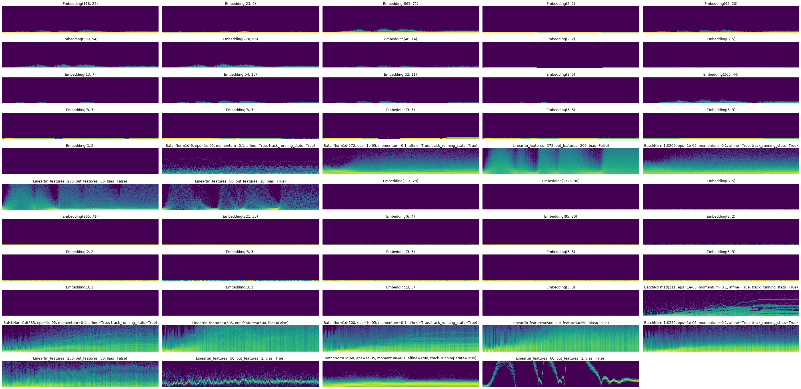
Thanks for the app name! Sorry I am at work, so I did those graph during lunch:

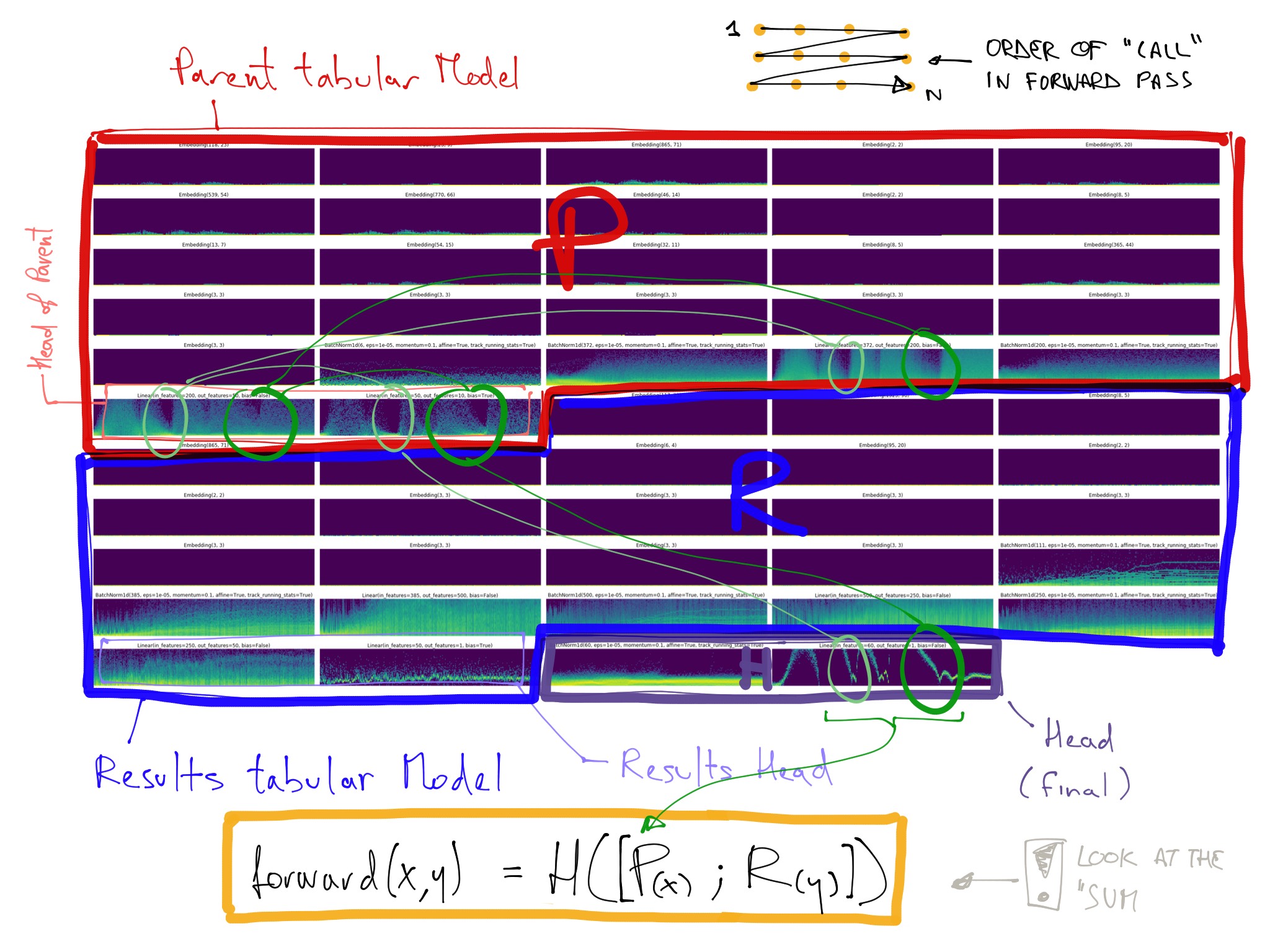
self.results (the TabularModel responsible to get the questionnaire into a feature vector)

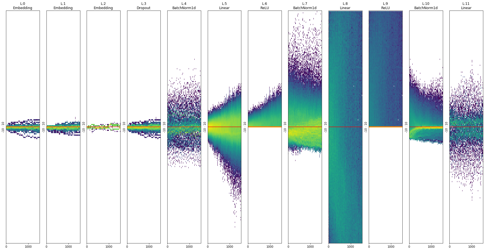
Then self.questions, the TabularModel called in a loop (one time for each questionnaire in the batch). We pass a batch of questions in this model). Replaced the BatchNorm by LayerNorm here:

self.attn, the MultiHeadSelfAttention layer. It doesn’t seem to be learning anything right now… Still have to figure this out.

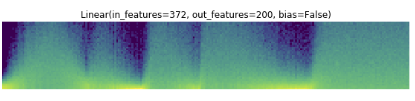
Then self.head which is responsible to predict the final prediction… I am confused, there doesn’t seem to be a lot of activities there:

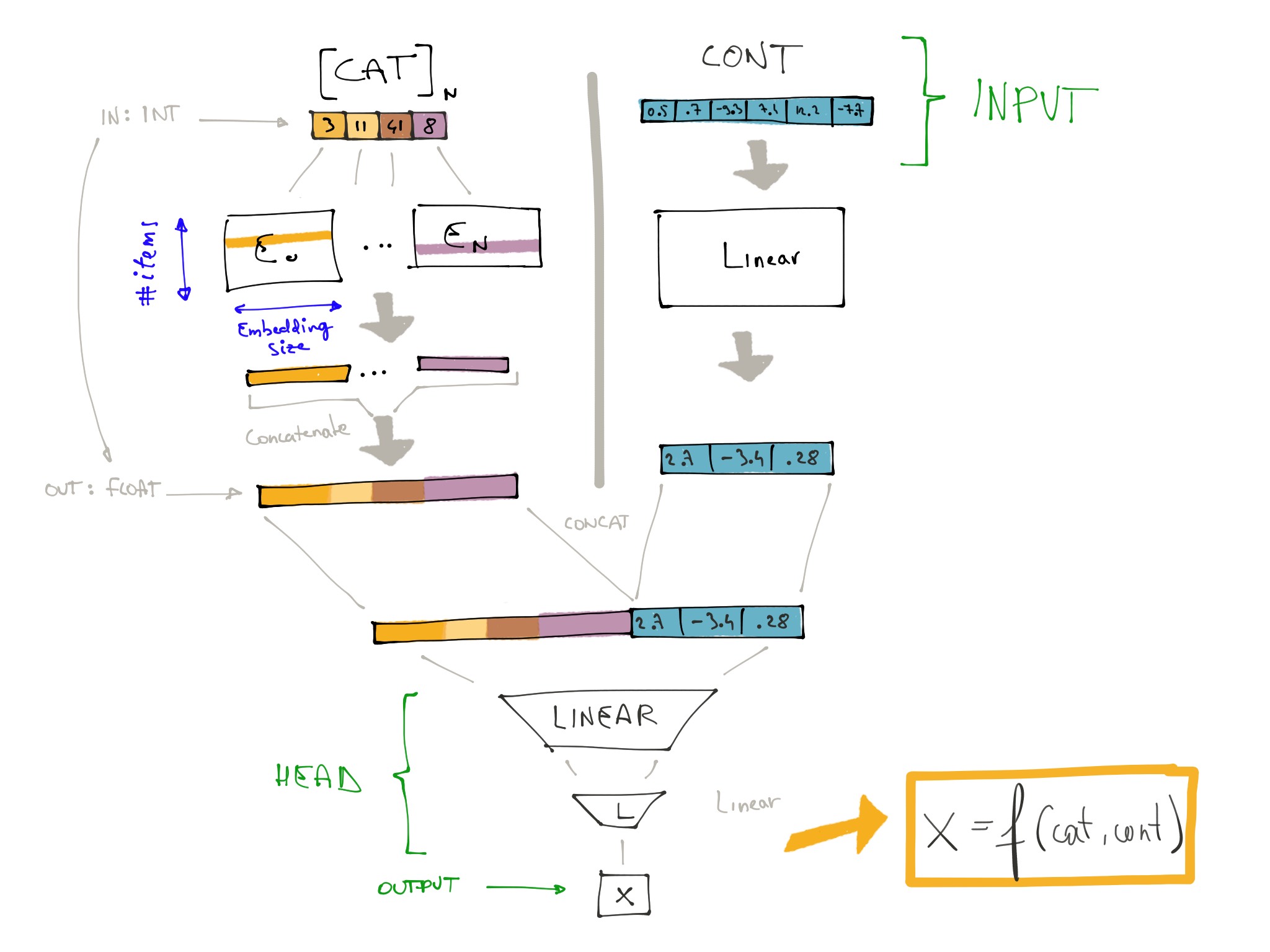
Here is the updated code for my mode, using attention:

results_emb_szs = get_emb_sz(results_tab)
questions_emb_szs = get_emb_sz(questions_tab)

class ParentChildModel(Module):
    def __init__(self):
        self.results = TabularModel(results_emb_szs, len(results_cont_names), 64, [512, 256], ps=[0.01, 0.1], embed_p=0.04, bn_final=True)
        self.questions = QuestionModel(questions_emb_szs, len(questions_cont_names), 1, layers=[512, 256, 64], ps=[0.01, 0.1, .1], embed_p=0.04, y_range=[-1,101])
    
        self.attn = MultiHeadAttention(1, 64, 64, 64)
        
        self.head = nn.Sequential(*[LinBnDrop(128, 1, p=0., bn=True), SigmoidRange(*[-1, 101])])
        
        for p in self.parameters():
            if p.dim() > 1:
                nn.init.kaiming_uniform_(p)

    def forward(self, data, children):
        parent_cat, parent_cont = data[0], data[1]
        results = self.results(parent_cat, parent_cont)
        
        questionScores = []
        batchQuestionMid = []
        lengths = []
        
        for children_cat, children_cont, length in children:
            result, mid = self.questions(children_cat[:length], children_cont[:length])
            result = result.squeeze()
            lengths += [length]
            batchQuestionMid += [F.pad(mid, pad=(0, 0, 0,children_cat.shape[0]-len(mid)), mode='constant', value=1e-7)]
            questionScores += [F.pad(result, pad=(0,1000-len(result)), mode='constant', value=1e-7)]
        
        lengths = torch.cat(lengths)
        batchQuestionMid = torch.stack(batchQuestionMid)
        
        mask = torch.arange(batchQuestionMid.shape[1]).repeat((batchQuestionMid.shape[0],1)).to(lengths.device) < lengths[:, None]
        mask = mask.unsqueeze(-1)
        
        batchQuestionMid, attention = self.attn(batchQuestionMid, batchQuestionMid, batchQuestionMid, mask)
        
        mid_merged = batchQuestionMid.sum(axis=1)
        
        concat = torch.cat([results, mid_merged], axis=1)
        results = self.head(concat)
        
        questionScores = torch.stack(questionScores, dim=0)
        return results, questionScores

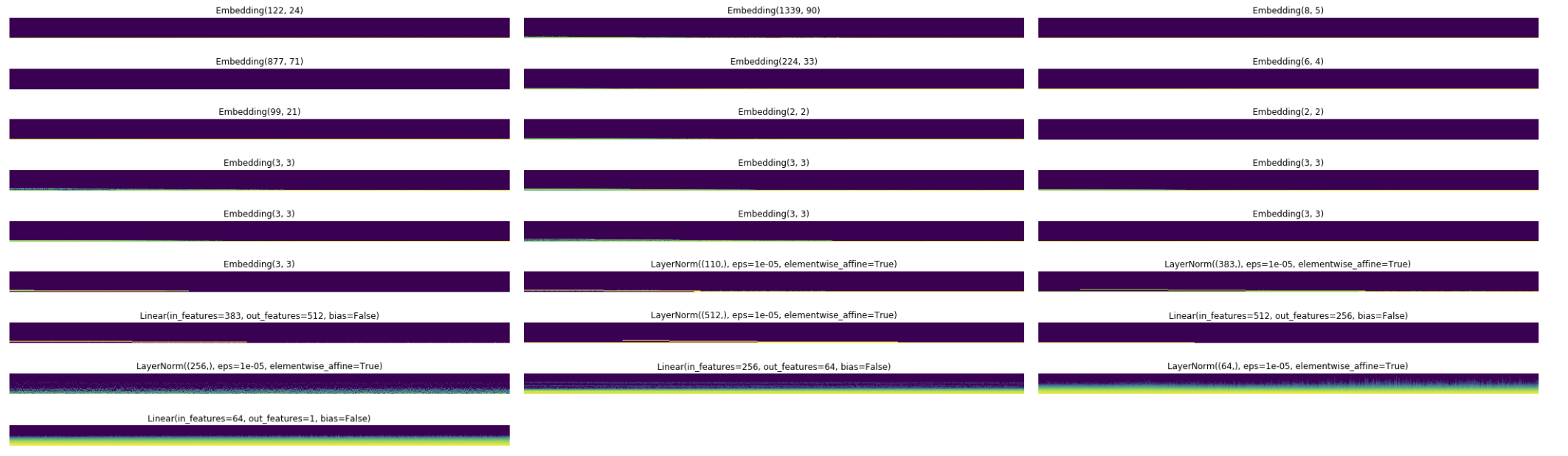
And a more complete export of the structure of the model:

ParentChildModel(
  (results): TabularModel(
    (embeds): ModuleList(
      (0): Embedding(123, 24)
      (1): Embedding(24, 9)
      (2): Embedding(877, 71)
      (3): Embedding(2, 2)
      (4): Embedding(99, 21)
      (5): Embedding(549, 55)
      (6): Embedding(782, 67)
      (7): Embedding(46, 14)
      (8): Embedding(2, 2)
      (9): Embedding(8, 5)
      (10): Embedding(13, 7)
      (11): Embedding(54, 15)
      (12): Embedding(32, 11)
      (13): Embedding(8, 5)
      (14): Embedding(365, 44)
      (15): Embedding(3, 3)
      (16): Embedding(3, 3)
      (17): Embedding(3, 3)
      (18): Embedding(3, 3)
      (19): Embedding(3, 3)
      (20): Embedding(3, 3)
    )
    (emb_drop): Dropout(p=0.04, inplace=False)
    (bn_cont): BatchNorm1d(6, eps=1e-05, momentum=0.1, affine=True, track_running_stats=True)
    (layers): Sequential(
      (0): LinBnDrop(
        (0): BatchNorm1d(376, eps=1e-05, momentum=0.1, affine=True, track_running_stats=True)
        (1): Dropout(p=0.01, inplace=False)
        (2): Linear(in_features=376, out_features=512, bias=False)
        (3): ReLU(inplace=True)
      )
      (1): LinBnDrop(
        (0): BatchNorm1d(512, eps=1e-05, momentum=0.1, affine=True, track_running_stats=True)
        (1): Dropout(p=0.1, inplace=False)
        (2): Linear(in_features=512, out_features=256, bias=False)
        (3): ReLU(inplace=True)
      )
      (2): LinBnDrop(
        (0): BatchNorm1d(256, eps=1e-05, momentum=0.1, affine=True, track_running_stats=True)
        (1): Linear(in_features=256, out_features=64, bias=False)
      )
    )
  )
  (questions): QuestionModel(
    (embeds): ModuleList(
      (0): Embedding(122, 24)
      (1): Embedding(1339, 90)
      (2): Embedding(8, 5)
      (3): Embedding(877, 71)
      (4): Embedding(224, 33)
      (5): Embedding(6, 4)
      (6): Embedding(99, 21)
      (7): Embedding(2, 2)
      (8): Embedding(2, 2)
      (9): Embedding(3, 3)
      (10): Embedding(3, 3)
      (11): Embedding(3, 3)
      (12): Embedding(3, 3)
      (13): Embedding(3, 3)
      (14): Embedding(3, 3)
      (15): Embedding(3, 3)
    )
    (emb_drop): Dropout(p=0.04, inplace=False)
    (bn_cont): LayerNorm((110,), eps=1e-05, elementwise_affine=True)
    (layers): Sequential(
      (0): LinLnDrop(
        (0): LayerNorm((383,), eps=1e-05, elementwise_affine=True)
        (1): Dropout(p=0.01, inplace=False)
        (2): Linear(in_features=383, out_features=512, bias=False)
        (3): ReLU(inplace=True)
      )
      (1): LinLnDrop(
        (0): LayerNorm((512,), eps=1e-05, elementwise_affine=True)
        (1): Dropout(p=0.1, inplace=False)
        (2): Linear(in_features=512, out_features=256, bias=False)
        (3): ReLU(inplace=True)
      )
      (2): LinLnDrop(
        (0): LayerNorm((256,), eps=1e-05, elementwise_affine=True)
        (1): Dropout(p=0.1, inplace=False)
        (2): Linear(in_features=256, out_features=64, bias=False)
        (3): ReLU(inplace=True)
      )
    )
    (layers2): Sequential(
      (0): LinLnDrop(
        (0): LayerNorm((64,), eps=1e-05, elementwise_affine=True)
        (1): Linear(in_features=64, out_features=1, bias=False)
      )
      (1): SigmoidRange(low=-1, high=101)
    )
  )
  (attn): MultiHeadAttention(
    (w_qs): Linear(in_features=64, out_features=64, bias=False)
    (w_ks): Linear(in_features=64, out_features=64, bias=False)
    (w_vs): Linear(in_features=64, out_features=64, bias=False)
    (fc): Linear(in_features=64, out_features=64, bias=False)
    (attention): ScaledDotProductAttention(
      (dropout): Dropout(p=0.1, inplace=False)
    )
    (dropout): Dropout(p=0.1, inplace=False)
    (layer_norm): LayerNorm((64,), eps=1e-06, elementwise_affine=True)
  )
  (head): Sequential(
    (0): LinBnDrop(
      (0): BatchNorm1d(128, eps=1e-05, momentum=0.1, affine=True, track_running_stats=True)
      (1): Linear(in_features=128, out_features=1, bias=False)
    )
    (1): SigmoidRange(low=-1, high=101)
  )
)

Took the time to inspect a bit what is going on with self.questions layer. It outputs almost always the same thing. It always output the same question score and the same middle layer vector values of length 64 that I use as feature vectors representing the questions.

So attention can’t really do it’s job after that. Well it attends to them all equally since they are the same, so in a sense it is doing its job haha.

1 Like