Help me understand Lesson 10 (Part 2)! :)

Hello friends, I’ve had troubles explaining my thoughts yesterday on twitter and I think that the a longer format of a post might be useful for me to express better! Plus, maybe I can spark an interesting discussion and we (or selfishly, I :innocent:) can learn something from it!

For context here is the twitter post from @radek (thanks for starting the discussion!) with replies from @jeremy in the comments!
I’m essentially having trouble sharing the idea that the convolutions described are wasteful …

First point : link reference in the video

Jeremy shows how for a 3x3 patch in the starting image (so 9 pixels, the image has only 1 channel), using 3x3 kernel and 8 filters you end up with 8 activations.
True, of course; the 9x8 matrix he shows is the “equivalent” matrix (wrt the 8 3x3 conv kernels) acting on the flattened 3x3 patch, that produce these 8 activations.

Jeremy says we’re just re-ordering / shuffling them, without doing any useful computation. I don’t think I can see it this way…

For fully connected layers I have the a similar intuition, you’re computing linear combinations (sorry, I should say affine transforms!) of your inputs and there you’d love to reduce the dimension, to find a lower dimensional space that contains the same info as the starting point but it’s easier to deal with.

But here we’re actually using convolutions, so the same 72 numbers are shifted around the all image, sharing information between the patches and producing correlated activation! You don’t want to go TOO SHALLOW or you’re not going to catch anything at all (because of all the correlations!). Think in the ‘limit’ if you had just one kernel that detect a particular type of edge, say this ‘’ … you’d be losing all the info about ‘/’ and ‘|’ and ‘-’ etc etc …

Moreover there’s this idea of the universal function approximations even for fully connected layers! In the limit for an infinite amount of filters, even a single fully connected layer should be able to approximate any function! So more is generally better!
We know now that deeper is surely more efficient than wider (as we introduce more non-linearities etc… etc…) but I don’t think we can dismiss the fact that wider still helps even if a bit counter-intuitive!

Am I missing something in what Jeremy is explaining here?

Second point video (rephrased a bit later here )

Switching to Imagenet models (which have 3 channels -> 27 weights in the each kernel), Jeremy sais that going from 27 to 32 is “wasting information” because we’re diluting the information we had at the start.
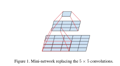
He proposes then to use a 5x5 kernel at the beginning of the net, which makes the transformation from 75 input (5x5x3) to 32 activations.

In contrast ResNet-C in the Bag of Tricks paper, borrowing from the Inception architecture, actually argues in favor of multiple small kernels at the stem.

img5x5to3x3

Quoting from Szegedy et al. 2016

[…] we can use the computational and memory savings (due to the factorization the convolutions) to increase the filter-bank sizes of our network while maintaining our ability to train each model replica on a single computer

emphasis mine. So in their idea a higher number of filters would actually be better, which sort of bounce back to the “universal approximator” idea I brought out before!

The general idea in the lesson is nonetheless that we shouldn’t be using a lot of filters at the start (In He et al 2018 they actually go back to increasing the number filters more gradually, using 32 for the very first 2 convolutions and then going to 64), which I agree with, but for different reasons that has more to do with efficiency than anything else!

I think you want to gradually increase the portion of the image you’ve looked at and the number of filters/features ‘together’, because the 3x3 kernels look at a very small part of the image and (in that space, i.e. the original image) there’s only so much you can “catch” with a 3x3 kernel (edges, small corners, … ) and it’s better in my opinion to use more computations at higher layers where the receptive fields capture representations of bigger patches of the original image!

This has more to do with the “semantics” of the image classification (or representation rather) rather then the actual computations done. It has to do with the fact that we’re talking about the actual input image and not just a 1 x width x height tensor of activations of some kind! (*)

To make what I mean clearer as in what I find unsettling about the lesson, in principle you could “shift Jeremy’s argument up a few layers” and take any 3x3 patch of activations from below in the network. By his arguments it seems that when using a 3x3 convolution we ought to use max 8 filters regardless of where we are in the network, because we’d end up with a similar amount of activations as we have inputs; think of a non-bottleneck layer in ResNet, where you go for example from a X channels “image” made of activations from below to another X channel output … with padding the 2 activations will actually have the same dimensions, but I don’t think we’re doing nothing there, nor I think that a possible intermediate ReLU is doing all the work!

But again I’m not sure Jeremy is implying that at all, I’m just extrapolating here! Maybe afterall my thinking is not so different from Jeremy’s, just expressed in a different way :slight_smile:

I find it intriguing though that the idea of using small 3x3 kernels at the beginning of the net stemmed from a computational point of view (same receptive field but lower num of parameters) but has since been shown to work well in practice. I find myself having to rethink this every time every time I do image classification because I struggle intuitively with the idea that a 3x3 kernel could actually capture anything meaningful from an image ( I mean 9 pixels!! ), especially for more structured “images” like spectrograms or piano rolls ( I like to deal with sound and music, you should definitely talk about the fastai audio at some point! :smiley: ) … but they always work best! I wonder where is the magical intuition for that!

Aaaanyway, this became much longer that I thought! I’m glad I didn’t decide to make it into a twitter thread!
What are your thoughts?

Anybody can help me clarify / discuss / elaborate the points I made above? :slight_smile:


Sidenote: Thinking back I don’t know what I was referring to when I said “compression” in my tweet; maybe to the fact that using the same 72 weights across the image you get as output correlated activations that are sharing some structure, so “compressible” rather than “compressed”. It might just have been the wrong word (Friday night) altogether! Sorry!

(*) I find really fascinating in NNs works like DeconvNets and derivations exactly because they give us clues of this “semantics” for the intermediate layers! :slight_smile:

4 Likes

Sorry, I don’t think I can fully address your concerns, but here are some bits of thought that maybe can be helpful

Convolutions perform a subset of the operation that an FC layer does. That might be useful for building up intuition about the differences between FCs and conv layers (~ convs are like FC but on values that are more spatially related, closer together)

FCs would do linear combination if it was not for the fact that we always follow an FC layer with a non-linearity, that might play a bit into what they do in the bigger picture.

That is an extremely tricky perspective to adopt, that bit on the universal function approximator. In theory that is the case, but I think in practice due to resource / algorithmic constraints we need to consider how best we can make the task easy for our NN.

Anyhow, this is pure speculation :slightly_smiling_face: Hopefully one day I will learn to not talk about things I don’t 100% get on the Internet, but that day has not arrived yet! :slight_smile: We can only be hopeful though and as such here are my thoughts for what its worth!

2 Likes

Completely agree, that’s why I said that in general we know that (for a fixed computational budget especially) going deeper is a better idea than going wider! It was just to say that in principle I don’t think those would be “lost computations”, but it’s probably true that they’d be “wasted”!

I think the takeaway here is rather than the more we open-mindedly {}^1 talk and get people to talk about things we don’t fully understand, the more we understand in the long run! This is the definition of constructive discussion to me!


{}^1: is this even a word? :sweat_smile:

2 Likes

No not at all! The discussion in the video was about single channel inputs. However in the later layers of the network you never have a single channel input. In fact, most architectures double the number of filters after each downsampling. The resnet blocks, for instance, have 64-512 filters. So at the last layer each conv at each grid position is adding up 33512 = 4608 multiplications.

2 Likes

… and resulting only in 512 activations for that patch, so that’s true that we’re summarizing something there!

I’m still struggling with the stem part, but I think talking about it has helped me a lot in clearing some of the confusion I had, thanks!

1 Like

For another (hand-wavy) perspective if it helps: to me the deeper input stem can better featurize the inputs. In the original network, the 7x7 convolution slides over a good portion of the input (much more than a 3x3 does at least). Then there is a max-pool soon after.

That means a lot of input is “consumed” in the earliest parts of the network. Max-pooling also technically breaks the sampling theorem. Although this is something deep nets seem to power through (maybe they get more information from correlations in the alias images?). So the combo of large convolutions with maxpooling leads to a smaller, potentially noisier feature map.

The changed BoT input stem could give the network more expressibility for the inputs with its added depth. That also means the residual blocks would see a richer set of feature maps.

Too many words to say:

  1. Better featurization from deeper stem
  2. Deeper feature maps potentially less sensitive to max-pooling aliasing
2 Likes

I completely agree on this points! It also brings computational advantages, so I don’t see a reason why not use deeper stacks of smaller kernels!

This is precisely why I’m confused at video recommending seemingly larger kernel sizes and relatively low number of filters … it seems to me that while this might make intuitive sense, it has been shown to be otherwise both

  • theoretically ; universal function approximation and related, for example (although again you probably don’t want to go TOO wide either at the start)
  • and empirically; the stem being the only part of the network in both ResNet and Bag of Tricks paper where we increase the number of filters at a much higher rate than we’re downsampling the images height and width!
1 Like

@marco_b thanks for creating this discussion, as I had similar reservations when I listened to the video.

I completely agree with your first point.

As to your second point:

Here’s the magic of why a 5x5 convolution can be replaced by applying two consecutive 3x3 convolutions :

Consider a one-dimensional toy example ‘image’ of 5 pixels in a row, labeled A, B, C, D, and E.

A 3x3 conv on ABCDE produces outputs

G(A,B,C) , H(B,C,D), and I(C,D,E) – where my notation G(A,B,C) means that G is a function of A, B, and C

Applying a second 3x3 conv on outputs GHI mixes them to produce an output
J(G,H,I) – which is a function of all 5 pixels ABCDE!

So: two consecutive 3x3 convs is equivalent in ‘effective range’ to a 5x5 conv, i.e. it looks for structure in image patches of 5x5 pixels. Additionally it requires only 3x3 + 3x3 = 18 weights, whereas a 5x5 convolution has 25 weights!

IN the same way, applying a third consecutive 3x3 conv leads to an effective range of 7x7 pixels – see if you can convince yourself of this! And instead of 49 weights, you only need 3x3 + 3x3 + 3x3 = 27!

And to blow your mind even further, a 3x3 convolution can be replace by two consecutive 2x2 convolutions, which covers the same 3x3 area on the image with 11% fewer weights!

So all convolutions could in principle be replaced by serial combinations of 2x2 convolutions!

I think the problem we are having is that the video is a bit unclear; I didn’t immediately understand Jeremy’s point either.

1 Like

That’s exactly right, especially in terms of ‘receptive field’ / ‘effective range’ / ‘pixels-in-the-input-image-it-looks-at’ ! As you mention, we also get something cheaper to compute, and that’s why the combination of multiple 3x3 it’s so commonly used!

What I don’t understand yet is this:

Why don’t practitioners break every convolution down into combinations of 2x2 convolutions?

Perhaps the answer is that the serial application of two 2x2 convolutions is slower than a single 3x3 convolution, so you’d have to trade off speed to get the 11% reduction in weights. (?)

1 Like

I had a similar question some time ago and found a lot of good answers here.

The short of it is part historical part convenience of implementation.
For the latter, think about what happens to padding with even-sized convolutions for example :slight_smile:

I think that having a ‘center pixel’ is simply easier both to conceptualize and to code efficiently …

1 Like

While both 1 3x3 and 2 2x2 look at a patch of same size (they have the same receptive field) they are not equivalent in what they can learn.

My guess would be that empirically 3x3 convs perform better :slight_smile: Still, an experiment juxtaposing a simple CNN built with 3x3 convs and and one with a double amount of 2x2 convs would probably make for an interesting read :slight_smile:

1 Like

The same is true of a single 5x5 convolution vs. two consecutive 3x3 convolutions, i.e. the 5x5 can ‘learn more’. Yet two 3x3 convs are found to be at least as effective as a single 5x5 conv.

Yes, that is true. I’m just not sure if the effect would hold going deeper and narrower to 2x2 from 3x3.

I’m not exactly sure if 5x5 can learn more - on one hand, it will have more parameters to work with, on the other it will lack the depth of 2 3x3 (depth is useful for learning more interesting nonlinearities).

Despite the effective receptive fields being the same, both will learn something different.

1 Like

Applying BatchNorm and non-linearities in-between the layers changes things a bit, but the smaller (serial) convolutions in essence “tie” some of the parameters together, similarly to for example hierarchical/multilevel models.

So yes in theory larger convolutions have more “freedom” i.e. more parameters that they can learn to combine pixel together, but in practice smaller convolutions might very well perform as well as if not better thanks to the additional non-linearity (and save some computations in the process).

I suspect that we don’t have much literature on 2x2 kernels because of the weirdness connected with their implementation! Another example on top of my mind is: think what happens when you want to reduce the image/activation size, with 3x3 convolutions you apply a stride of 2, you half the height and width of the output layer (wrt inputs) but you still retain some overlap between consecutive kernels (which you want in order to maintain some correlation between the activations)!

If you use a 2x2 kernel there’s no way to have overlapping applications that also reduce the image size (other than by 1 pixel at a time if you don’t pad one side [if you pad both you actually increase the size by 1)!!

Probably the marginal (if any) gain associated with it didn’t warrant any real-work application, contrary to the gains for 3x3 VS bigger 5x5 or 7x7 kernels…

1 Like

Hi @radek I was thinking that the number of weights is the only criterion for learning, but you correctly point out that the depth is also a factor for learning nonlinearities.

But then, could you explain why you think that a 3x3 conv can learn “more” than two consecutive 2x2 convs?

But the very next layer in 2x2 will “do the overlapping”. e.g. instead of a single 3x3 Conv with stride 2 you would have a 2x2 Conv with stride 2 followed by a 2x2 Conv with stride 1.

1 Like

Without non-linearities sure, but imagine if one of the activations is zeroed by a ReLU!

I’m not arguing they have no place, but as I’ve written before I think that if you add up this ‘tricky bits’ , the historic perspective and the added computations (mainly for batchnorm, relu is quite cheap, plus the sequential computation) I can see why even if you’d have a little reduction in weights the community hasn’t really exploited this additional factorization.

I agree it would be interesting to see if there’s a difference, but I suspect that if there is one it won’t be very relevant… I might explore the idea a little if I find the time this week.

Also a 2x2 kernel is very restrictive in terms of what it can represent (even if we’re dealing with continuous weights, you don’t want two kernels to pick up the same thing, just slightly scaled differently), so maybe it’ll warrant added consideration into the useful filter sizes at this low kernel size, going back to point 1 of my post.

1 Like

Hm… Very good point, is it crazy to have a sequence of some convolutions without ReLU?

I’ll work on this rn actually, and will post results here :grin:

1 Like