Hi All,
There was a lot of material covered for lesson9. There’s a copy of the notes on my github : https://github.com/timdavidlee/fast_dl2
Otherwise, hope the notes are helpful.
[Update, i actually hit the character limit, so I’ve truncated some of the notes]
[Update: 4/8, applied jeremy’s edits]
Tim
%matplotlib inline
%reload_ext autoreload
%autoreload 2
import sys
sys.path.append('../')
from fastai.conv_learner import *
from fastai.dataset import *

from pathlib import Path
import json
from PIL import ImageDraw, ImageFont
from matplotlib import patches, patheffects

# check to make sure you set the device
torch.cuda.set_device(0)
Welcome to Lecture 9
Last Week: Largest Item Classifier
Last Week: Bbox only
Let’s Continue start with Single Object detecion
Load the data from last week, and global keys
-
PATH- is the location of the dataset -
JPEGS- images -
CSV- filenames and categorical labels
PATH = Path('data/pascal')
JPEGS = 'VOCdevkit/VOC2007/JPEGImages'
CSV = PATH/'tmp/lrg.csv'

IMAGES,ANNOTATIONS,CATEGORIES = ['images', 'annotations', 'categories']
FILE_NAME,ID,IMG_ID,CAT_ID,BBOX = 'file_name','id','image_id','category_id','bbox'
Show image function
def show_img(im, figsize=None, ax=None):
    if not ax: fig,ax = plt.subplots(figsize=figsize)
    ax.imshow(im)
    ax.get_xaxis().set_visible(False)
    ax.get_yaxis().set_visible(False)
    return ax
-
bb_hw= Convenience Function to swap the order of the coordinates (See lesson 8) -
draw_outline= adds a black border around any line. This ensures we can read it regardless of whether the background is light or dark. -
draw_rect= draw the bounding rectangle -
draw_text= write the text category on the image
def bb_hw(a): return np.array([a[1],a[0],a[3]-a[1],a[2]-a[0]])

def draw_outline(o, lw):
    o.set_path_effects([patheffects.Stroke(
        linewidth=lw, foreground='black'), patheffects.Normal()])

def draw_rect(ax, b):
    patch = ax.add_patch(patches.Rectangle(b[:2], *b[-2:], fill=False, edgecolor='white', lw=2))
    draw_outline(patch, 4)

def draw_text(ax, xy, txt, sz=14):
    text = ax.text(*xy, txt,
        verticalalignment='top', color='white', fontsize=sz, weight='bold')
    draw_outline(text, 1)
Load the 2007 training data in the json format
trn_j = json.load((PATH/'pascal_train2007.json').open())
trn_fns = dict((o[ID], o[FILE_NAME]) for o in trn_j[IMAGES])
cats = dict((o[ID], o['name']) for o in trn_j[CATEGORIES])
Our image data
trn_j.keys()
dict_keys(['images', 'type', 'annotations', 'categories'])
ID to picture file name
trn_fns[12]
'000012.jpg'
BB_CSV = PATH/'tmp/bb.csv'
Load the resnet model
f_model=resnet34
sz=224
bs=64

val_idxs = get_cv_idxs(len(trn_fns))
create transformations and image dataset:
-
sz= image size -
crop_type= this case we will not crop the image, since we might cut off objects we need to recognize around the edges, but it will ‘squish’ it into a square shape, since this is required by fastai( for now at least). -
tfm_y= this is the y transformation that will be adjusted
Objects:
-
tfms= transformations to apply -
md= dataset has the bounding box information -
md2= transformations to has the actual categorical labelings
tfms = tfms_from_model(f_model, sz, crop_type=CropType.NO, tfm_y=TfmType.COORD)
md = ImageClassifierData.from_csv(PATH, JPEGS, BB_CSV, tfms=tfms,
    continuous=True, val_idxs=val_idxs)

md2 = ImageClassifierData.from_csv(PATH, JPEGS, CSV, tfms=tfms_from_model(f_model, sz))
Let’s make a custom Datasets that will have a 2nd set of labels
The custom dataset will have the following structure:
**(md) Image - (md)Bounding Box - (md2) Label **
Note that the __getitem__() will return a concatenated tuple:
(x, (y1, y2))
def __getitem__(self, i):
    x,y = self.ds[i]
    return (x, (y,self.y2[i]))
class ConcatLblDataset(Dataset):
    def __init__(self, ds, y2): self.ds,self.y2 = ds,y2
    def __len__(self): return len(self.ds)

    def __getitem__(self, i):
        x,y = self.ds[i]
        return (x, (y,self.y2[i]))
Create training and test sets
trn_ds2 = ConcatLblDataset(md.trn_ds, md2.trn_y)
val_ds2 = ConcatLblDataset(md.val_ds, md2.val_y)
The image
val_ds2[0][0]
array([[[ 0.39125,  0.43014,  0.48172, ...,  0.17518,  0.32367,  0.40783],
        [ 0.51636,  0.44973,  0.59202, ...,  0.17386,  0.23164,  0.36722],
        [ 0.54416,  0.57267,  0.70099, ...,  0.05768,  0.2232 ,  0.35455],
        ...,
        [ 1.46039,  1.50291,  1.5195 , ...,  0.7803 ,  0.56716, -0.63922],
        [ 0.93739,  1.021  ,  1.15993, ...,  1.12806,  1.08947,  0.45857],
        [ 0.58584,  0.45245,  0.29605, ...,  1.00028,  0.92495,  0.82729]],

       [[ 0.24041,  0.31444,  0.41422, ...,  0.33162,  0.47052,  0.54764],
        [ 0.39737,  0.42156,  0.57304, ...,  0.33887,  0.38799,  0.52038],
        [ 0.52462,  0.58245,  0.67485, ...,  0.2519 ,  0.40003,  0.51502],
        ...,
        [ 1.47208,  1.50185,  1.50771, ...,  0.60917,  0.44337, -0.73978],
        [ 0.84169,  0.94566,  1.06783, ...,  0.97373,  1.01637,  0.39674],
        [ 0.47731,  0.36442,  0.1823 , ...,  0.85592,  0.85008,  0.75529]],

       [[ 0.63094,  0.76758,  0.91924, ...,  0.46997,  0.58218,  0.63571],
        [ 0.86685,  0.89343,  1.08916, ...,  0.4597 ,  0.4921 ,  0.60825],
        [ 0.96684,  1.00092,  1.07853, ...,  0.35109,  0.50631,  0.63579],
        ...,
        [ 1.56056,  1.59266,  1.60554, ...,  0.54531,  0.38118, -0.79327],
        [ 0.92625,  1.02055,  1.14452, ...,  0.91826,  0.93747,  0.31286],
        [ 0.56966,  0.44559,  0.26428, ...,  0.8008 ,  0.77093,  0.67405]]], dtype=float32)
The Bounding box and category
val_ds2[0][1]
(array([ 0., 49., 205., 180.], dtype=float32), 14)
Replace the md dataset with the new 2 labeled dataset
md.trn_dl.dataset = trn_ds2
md.val_dl.dataset = val_ds2
We have to denormalize the images from the dataloader before they can be plotted.
x,y=next(iter(md.val_dl))

ima=md.val_ds.ds.denorm(to_np(x))[1]
b = bb_hw(to_np(y[0][1])); b
array([ 1., 63., 222., 159.], dtype=float32)
ax = show_img(ima)
draw_rect(ax, b)
draw_text(ax, b[:2], md2.classes[y[1][1]])
Add a custom head to the end of resnet34
We need one output activation for each class (for its probability) plus one for each bounding box coordinate. We’ll use an extra linear layer this time, plus some dropout, to help us train a more flexible model.
head_reg4 = nn.Sequential(
    Flatten(),
    nn.ReLU(),
    nn.Dropout(0.5),
    nn.Linear(25088,256),
    nn.ReLU(),
    nn.BatchNorm1d(256),
    nn.Dropout(0.5),
    nn.Linear(256,4+len(cats)),
)
models = ConvnetBuilder(f_model, 0, 0, 0, custom_head=head_reg4)

learn = ConvLearner(md, models)
learn.opt_fn = optim.Adam
Definte a Loss, L1 regularization, and Accuracy helper functions
Loss function
-
bb_i = F.sigmoid(bb_i)*224- force the value between 0 and 1 (times 224). This is to force the data into a specific range of values - Where to put
batch_norm? Recommended to put it after relu, so you keep the ability to make negative numbers. -
L1 loss + Cross Entropy Loss=F.l1_loss(bb_i, bb_t) + F.cross_entropy(c_i, c_t)*20. Thex20is approximated to ensure that the two losses are on the same scale
def detn_loss(input, target):
    bb_t,c_t = target
    bb_i,c_i = input[:, :4], input[:, 4:]
    bb_i = F.sigmoid(bb_i)*224
    # I looked at these quantities separately first then picked a multiplier
    #   to make them approximately equal
    return F.l1_loss(bb_i, bb_t) + F.cross_entropy(c_i, c_t)*20

def detn_l1(input, target):
    bb_t,_ = target
    bb_i = input[:, :4]
    bb_i = F.sigmoid(bb_i)*224
    return F.l1_loss(V(bb_i),V(bb_t)).data

def detn_acc(input, target):
    _,c_t = target
    c_i = input[:, 4:]
    return accuracy(c_i, c_t)

learn.crit = detn_loss
learn.metrics = [detn_acc, detn_l1]
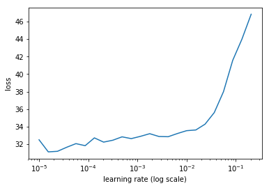
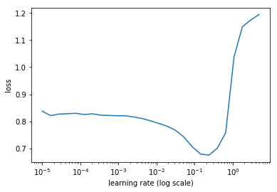
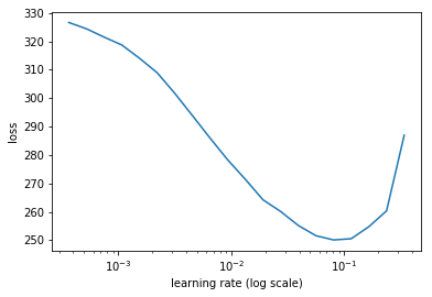
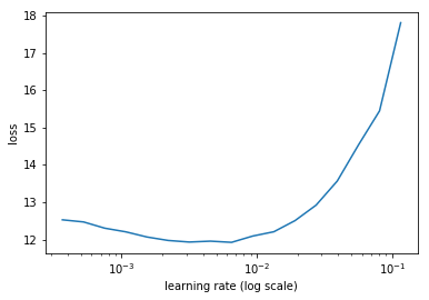
With the metrics defined, we find the learning rate
learn.lr_find()
learn.sched.plot()
97%|█████████▋| 31/32 [00:09<00:00, 3.19it/s, loss=524]
Set the rate
lr=1e-2
Fit the Model
learn.fit(lr, 1, cycle_len=3, use_clr=(32,5))
epoch      trn_loss   val_loss   detn_acc   detn_l1
    0      73.80378   43.574409  0.813852   31.699385
    1      51.747788  37.229919  0.819561   25.624957
    2      41.568981  35.318695  0.82497    24.513911


[35.318695, 0.8249699547886848, 24.51391077041626]
Save our Model
learn.save('reg1_0')
Freeze everything except the last two layers
learn.freeze_to(-2)
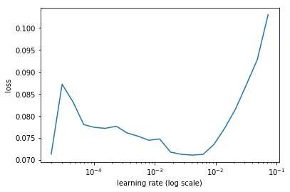
#### Setting learning rates
lrs = np.array([lr/100, lr/10, lr])
learn.lr_find(lrs/1000)
learn.sched.plot(0)
91%|█████████ | 29/32 [00:08<00:00, 3.36it/s, loss=230]
learn.fit(lrs/5, 1, cycle_len=5, use_clr=(32,10))
epoch      trn_loss   val_loss   detn_acc   detn_l1
    0      18.630316  36.514301  0.791466   21.233154
    1      19.990961  33.011433  0.81881    20.244233
    2      18.506014  31.954967  0.820763   19.621269
    3      16.846955  31.920164  0.81881    19.204269
    4      15.234001  31.665308  0.819261   18.943963


[31.665308, 0.8192608207464218, 18.943962812423706]
learn.save('reg1_1')
learn.load('reg1_1')
learn.unfreeze()
learn.fit(lrs/10, 1, cycle_len=10, use_clr=(32,10))
epoch      trn_loss   val_loss   detn_acc   detn_l1
    0      13.102859  30.631477  0.817758   18.990284
    1      13.380544  32.969467  0.810397   19.570258
    2      13.436793  32.149635  0.821214   19.051544
    3      12.934334  31.497986  0.83729    18.988035
    4      12.444968  32.228378  0.819261   18.880555
    5      11.878257  32.434448  0.809044   18.574428
    6      11.490413  31.936653  0.822716   18.974106
    7      10.877252  31.002441  0.832933   18.324932
    8      10.552304  30.984261  0.832933   18.481523
    9      10.308766  31.074959  0.81881    18.369649


[31.074959, 0.8188100978732109, 18.369649052619934]
learn.save('reg1')
learn.load('reg1')
y = learn.predict()
x,_ = next(iter(md.val_dl))
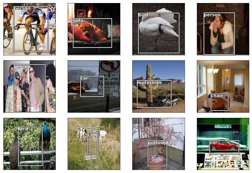
Big Idea
Figuring out what hte main object in an image is, that is the difficult task. Finding the bounding box is the easier part. So a model that has two do both, the tasks inform each other since they share some concept together. As a result, they should share some of the layers of the network together.
from scipy.special import expit
fig, axes = plt.subplots(3, 4, figsize=(12, 8))
for i,ax in enumerate(axes.flat):
    ima=md.val_ds.ds.denorm(to_np(x))[i]
    bb = expit(y[i][:4])*224
    b = bb_hw(bb)
    c = np.argmax(y[i][4:])
    ax = show_img(ima, ax=ax)
    draw_rect(ax, b)
    draw_text(ax, b[:2], md2.classes[c])
plt.tight_layout()
Clipping input data to the valid range for imshow with RGB data ([0..1] for floats or [0..255] for integers).
Checkout the Multi Label Classification
The notebook is posted link
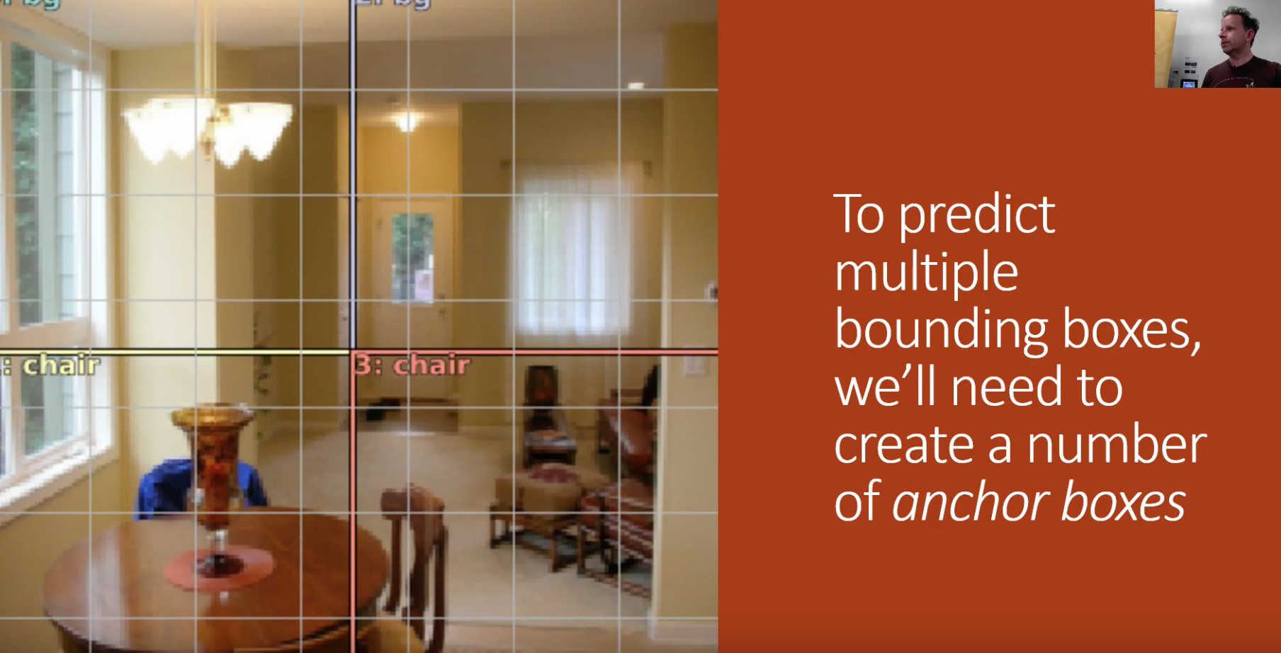
Finding multiple objects in a picture

Using the SSD Approach, we will now have a grid
So each Conv quadrant will be responsible for each part of the image. Why do we want each Convolution to be responsible for each part of the image? A concept called receptive field. Throughout your convolution layers, each piece of your tensor, has a receptive field.
Let’s look at Microsoft Excel
Our image went through a 3x3 kernel (right)
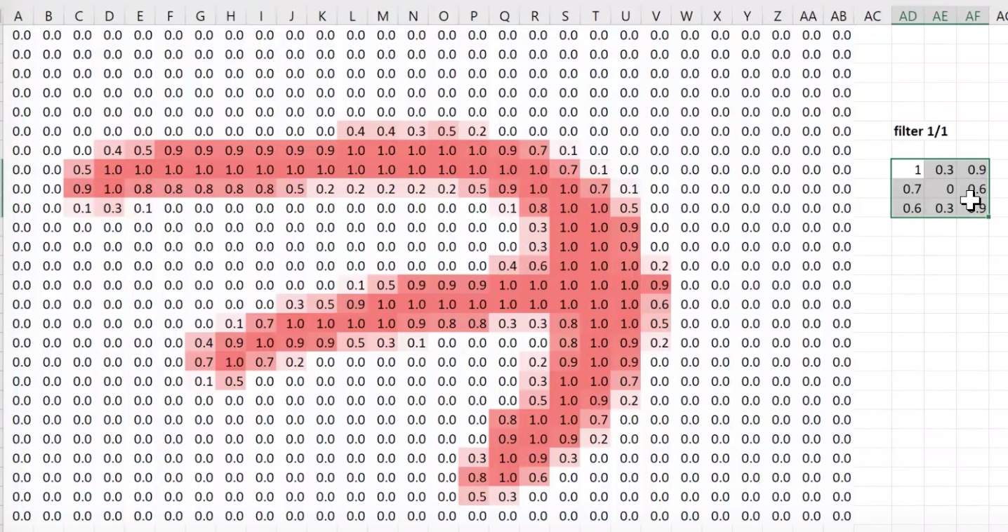
Created a two channel output
Then went through another channel output into max pooling (sparse area)
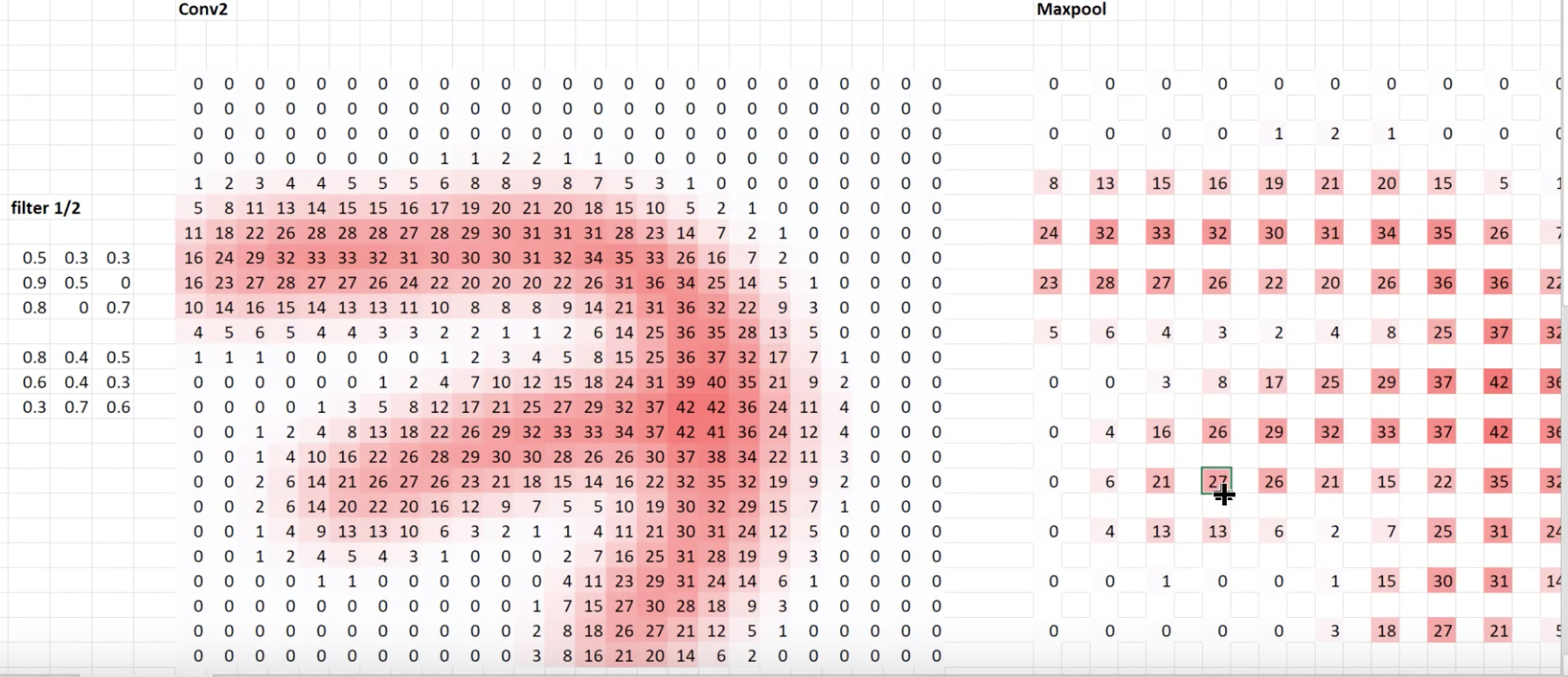
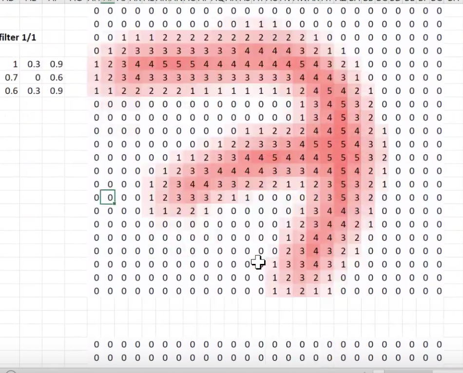
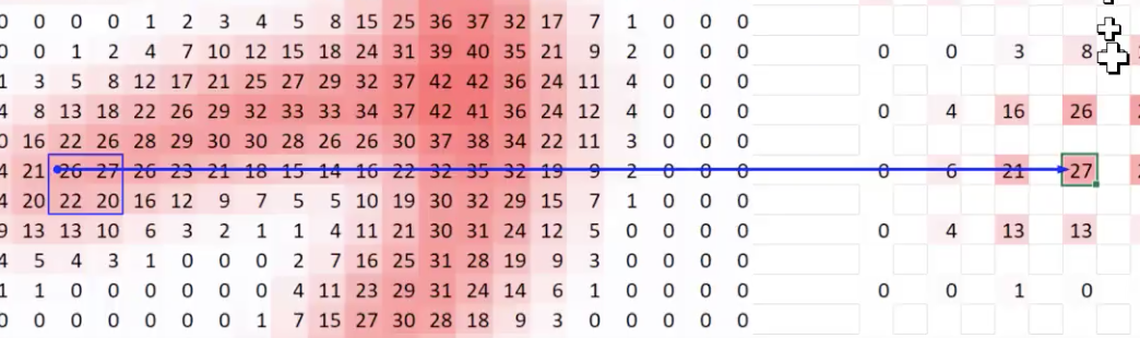
If we trace one of the maxpool steps (pretend its a Conv2D stride 2 layer) backwards:
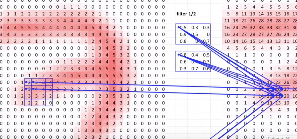
Tracing back even farther:
Tracing back to the source image:
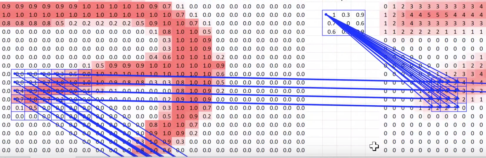
The pixels in the middle have a lot of connections, and the edges don’t have as many. The center of the box has more dependencies. This is critically important for understanding convolution receptive fields.
%matplotlib inline
%reload_ext autoreload
%autoreload 2
import sys
sys.path.append('../')
from fastai.conv_learner import *
from fastai.dataset import *

from pathlib import Path
import json
from PIL import ImageDraw, ImageFont
from matplotlib import patches, patheffects

# check to make sure you set the device
torch.cuda.set_device(0)
Setup Globals
PATH = Path('data/pascal')
trn_j = json.load((PATH / 'pascal_train2007.json').open())
IMAGES,ANNOTATIONS,CATEGORIES = ['images', 'annotations', 'categories']
FILE_NAME,ID,IMG_ID,CAT_ID,BBOX = 'file_name','id','image_id','category_id','bbox'

cats = dict((o[ID], o['name']) for o in trn_j[CATEGORIES])
trn_fns = dict((o[ID], o[FILE_NAME]) for o in trn_j[IMAGES])
trn_ids = [o[ID] for o in trn_j[IMAGES]]

JPEGS = 'VOCdevkit/VOC2007/JPEGImages'
IMG_PATH = PATH/JPEGS
Define Common Functions (very similar to the first pascal model)
def get_trn_anno():
    trn_anno = collections.defaultdict(lambda:[])
    for o in trn_j[ANNOTATIONS]:
        if not o['ignore']:
            bb = o[BBOX]
            bb = np.array([bb[1], bb[0], bb[3]+bb[1]-1, bb[2]+bb[0]-1])
            trn_anno[o[IMG_ID]].append((bb,o[CAT_ID]))
    return trn_anno

def show_img(im, figsize=None, ax=None):
    if not ax: fig,ax = plt.subplots(figsize=figsize)
    ax.imshow(im)
    ax.set_xticks(np.linspace(0, 224, 8))
    ax.set_yticks(np.linspace(0, 224, 8))
    ax.grid()
    ax.set_yticklabels([])
    ax.set_xticklabels([])
    return ax

def draw_outline(o, lw):
    o.set_path_effects([patheffects.Stroke(
        linewidth=lw, foreground='black'), patheffects.Normal()])

def draw_rect(ax, b, color='white'):
    patch = ax.add_patch(patches.Rectangle(b[:2], *b[-2:], fill=False, edgecolor=color, lw=2))
    draw_outline(patch, 4)

def draw_text(ax, xy, txt, sz=14, color='white'):
    text = ax.text(*xy, txt,
        verticalalignment='top', color=color, fontsize=sz, weight='bold')
    draw_outline(text, 1)

def bb_hw(a): return np.array([a[1],a[0],a[3]-a[1],a[2]-a[0]])

def draw_im(im, ann):
    ax = show_img(im, figsize=(16,8))
    for b,c in ann:
        b = bb_hw(b)
        draw_rect(ax, b)
        draw_text(ax, b[:2], cats[c], sz=16)

def draw_idx(i):
    im_a = trn_anno[i]
    im = open_image(IMG_PATH/trn_fns[i])
    draw_im(im, im_a)
Setup Multiclass
trn_anno = get_trn_anno()
MC_CSV = PATH/'tmp/mc.csv'

mc = [set([cats[p[1]] for p in trn_anno[o]]) for o in trn_ids]
mcs = [' '.join(str(p) for p in o) for o in mc]

df = pd.DataFrame({'fn': [trn_fns[o] for o in trn_ids], 'clas': mcs}, columns=['fn','clas'])
df.to_csv(MC_CSV, index=False)
df.head()
.dataframe tbody tr th {
    vertical-align: top;
}

.dataframe thead th {
    text-align: right;
}
| fn | clas | |
|---|---|---|
| 0 | 000012.jpg | car |
| 1 | 000017.jpg | person horse |
| 2 | 000023.jpg | bicycle person |
| 3 | 000026.jpg | car |
| 4 | 000032.jpg | person aeroplane |
Setup Resnet Model and Train
f_model=resnet34
sz=224
bs=64

tfms = tfms_from_model(f_model, sz, crop_type=CropType.NO)
md = ImageClassifierData.from_csv(PATH, JPEGS, MC_CSV, tfms=tfms)
learn = ConvLearner.pretrained(f_model, md)
learn.opt_fn = optim.Adam
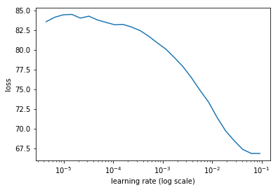
# find learning rate
lrf=learn.lr_find(1e-5,100)
# plot the learning rate to visually choose
learn.sched.plot(0)
# select learning rate
lr = 2e-2
# fit the model
learn.fit(lr, 1, cycle_len=3, use_clr=(32,5))
epoch      trn_loss   val_loss   <lambda>
    0      1.326271   16.738022  0.394231


epoch      trn_loss   val_loss   <lambda>
    0      0.326659   0.138878   0.954184
    1      0.174125   0.078377   0.973558
    2      0.11821    0.074982   0.974654


[0.07498233, 0.9746544435620308]
# define learning rates to search
lrs = np.array([lr/100, lr/10, lr])

# freeze the model till teh last 2 steps as before:
learn.freeze_to(-2)

# find the optimal learning rate again
learn.lr_find(lrs/1000)
learn.sched.plot(0)

# refit the model
learn.fit(lrs/10, 1, cycle_len=5, use_clr=(32,5))
 81%|████████▏ | 26/32 [00:07<00:01,  3.42it/s, loss=0.33]


epoch      trn_loss   val_loss   <lambda>
    0      0.070927   0.081387   0.972078
    1      0.052779   0.078058   0.974429
    2      0.038978   0.078155   0.974745
    3      0.027514   0.074822   0.977141
    4      0.019513   0.075868   0.977652


[0.075868085, 0.9776517376303673]
Save the model
learn.save('mclas')
learn.load('mclas')
multiple Bbox per cell
CLAS_CSV = PATH/'tmp/clas.csv'
MBB_CSV = PATH/'tmp/mbb.csv'

f_model=resnet34
sz=224
bs=64
Create Lookups and reference objects
-
mc- list of items found per image -
mcs- list of items found per image, but the ID -
id2cat- numeric value to category -
cat2id- category to id
mc = [[cats[p[1]] for p in trn_anno[o]] for o in trn_ids]
id2cat = list(cats.values())
cat2id = {v:k for k,v in enumerate(id2cat)}
mcs = np.array([np.array([cat2id[p] for p in o]) for o in mc]); mcs
array([array([6]), array([14, 12]), array([ 1,  1, 14, 14, 14]), ..., array([17,  8, 14, 14, 14]),
       array([6]), array([11])], dtype=object)
# get cross validation ids
val_idxs = get_cv_idxs(len(trn_fns))
((val_mcs,trn_mcs),) = split_by_idx(val_idxs, mcs)
Create and Save multiple Bounding boxes
mbb = [np.concatenate([p[0] for p in trn_anno[o]]) for o in trn_ids]
mbbs = [' '.join(str(p) for p in o) for o in mbb]

df = pd.DataFrame({'fn': [trn_fns[o] for o in trn_ids], 'bbox': mbbs}, columns=['fn','bbox'])
df.to_csv(MBB_CSV, index=False)
df.head()
.dataframe tbody tr th {
    vertical-align: top;
}

.dataframe thead th {
    text-align: right;
}
| fn | bbox | |
|---|---|---|
| 0 | 000012.jpg | 96 155 269 350 |
| 1 | 000017.jpg | 61 184 198 278 77 89 335 402 |
| 2 | 000023.jpg | 229 8 499 244 219 229 499 333 0 1 368 116 1 2 ... |
| 3 | 000026.jpg | 124 89 211 336 |
| 4 | 000032.jpg | 77 103 182 374 87 132 122 196 179 194 228 212 ... |
Setup Dataset
aug_tfms = [RandomRotate(10, tfm_y=TfmType.COORD),
            RandomLighting(0.05, 0.05, tfm_y=TfmType.COORD),
            RandomFlip(tfm_y=TfmType.COORD)]
tfms = tfms_from_model(f_model, sz, crop_type=CropType.NO, tfm_y=TfmType.COORD, aug_tfms=aug_tfms)
md = ImageClassifierData.from_csv(PATH, JPEGS, MBB_CSV, tfms=tfms, continuous=True, num_workers=4)
Create our Dataset with 2 associated Labels
class ConcatLblDataset(Dataset):
    def __init__(self, ds, y2):
        self.ds,self.y2 = ds,y2
        self.sz = ds.sz
    def __len__(self): return len(self.ds)

    def __getitem__(self, i):
        x,y = self.ds[i]
        return (x, (y,self.y2[i]))
trn_ds2 = ConcatLblDataset(md.trn_ds, trn_mcs)
val_ds2 = ConcatLblDataset(md.val_ds, val_mcs)
md.trn_dl.dataset = trn_ds2
md.val_dl.dataset = val_ds2
Setup some plotting functions
import matplotlib.cm as cmx
import matplotlib.colors as mcolors
from cycler import cycler

def get_cmap(N):
    color_norm  = mcolors.Normalize(vmin=0, vmax=N-1)
    return cmx.ScalarMappable(norm=color_norm, cmap='Set3').to_rgba

def show_ground_truth(ax, im, bbox, clas=None, prs=None, thresh=0.3):
    bb = [bb_hw(o) for o in bbox.reshape(-1,4)]
    if prs is None:  prs  = [None]*len(bb)
    if clas is None: clas = [None]*len(bb)
    ax = show_img(im, ax=ax)
    for i,(b,c,pr) in enumerate(zip(bb, clas, prs)):
        if((b[2]>0) and (pr is None or pr > thresh)):
            draw_rect(ax, b, color=colr_list[i%num_colr])
            txt = f'{i}: '
            if c is not None: txt += ('bg' if c==len(id2cat) else id2cat[c])
            if pr is not None: txt += f' {pr:.2f}'
            draw_text(ax, b[:2], txt, color=colr_list[i%num_colr])

num_colr = 12
cmap = get_cmap(num_colr)
colr_list = [cmap(float(x)) for x in range(num_colr)]
View the Sample labels
x,y=to_np(next(iter(md.val_dl)))
x=md.val_ds.ds.denorm(x)

x,y=to_np(next(iter(md.trn_dl)))
x=md.trn_ds.ds.denorm(x)
fig, axes = plt.subplots(3, 4, figsize=(16, 12))
for i,ax in enumerate(axes.flat):
    show_ground_truth(ax, x[i], y[0][i], y[1][i])
plt.tight_layout()

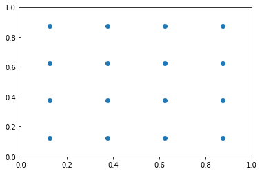
Make a model to predict what shows up in a 4x4 grid
-
anc_grid= how big of a square grid to make (subdivision) -
anc_offset= center offsets -
anc_x= x coordinates for centers -
anc_y= y coordinates for centers -
anc_ctrs- the actual coordinates for the grid centers -
anc_sizes- size of the quadrants
anc_grid = 4
k = 1

anc_offset = 1/(anc_grid*2)
anc_x = np.repeat(np.linspace(anc_offset, 1-anc_offset, anc_grid), anc_grid)
anc_y = np.tile(np.linspace(anc_offset, 1-anc_offset, anc_grid), anc_grid)

anc_ctrs = np.tile(np.stack([anc_x,anc_y], axis=1), (k,1))
anc_sizes = np.array([[1/anc_grid,1/anc_grid] for i in range(anc_grid*anc_grid)])
anchors = V(np.concatenate([anc_ctrs, anc_sizes], axis=1), requires_grad=False).float()

grid_sizes = V(np.array([1/anc_grid]), requires_grad=False).unsqueeze(1)
anchors
Variable containing:
 0.1250  0.1250  0.2500  0.2500
 0.1250  0.3750  0.2500  0.2500
 0.1250  0.6250  0.2500  0.2500
 0.1250  0.8750  0.2500  0.2500
 0.3750  0.1250  0.2500  0.2500
 0.3750  0.3750  0.2500  0.2500
 0.3750  0.6250  0.2500  0.2500
 0.3750  0.8750  0.2500  0.2500
 0.6250  0.1250  0.2500  0.2500
 0.6250  0.3750  0.2500  0.2500
 0.6250  0.6250  0.2500  0.2500
 0.6250  0.8750  0.2500  0.2500
 0.8750  0.1250  0.2500  0.2500
 0.8750  0.3750  0.2500  0.2500
 0.8750  0.6250  0.2500  0.2500
 0.8750  0.8750  0.2500  0.2500
[torch.cuda.FloatTensor of size 16x4 (GPU 0)]
plt.scatter(anc_x, anc_y)
plt.xlim(0, 1)
plt.ylim(0, 1);
#anchors = anchors.cpu(); grid_sizes = grid_sizes.cpu(); anchor_cnr = anchor_cnr.cpu()
def hw2corners(ctr, hw): return torch.cat([ctr-hw/2, ctr+hw/2], dim=1)
anchor_cnr = hw2corners(anchors[:,:2], anchors[:,2:])
anchor_cnr
Variable containing:
 0.0000  0.0000  0.2500  0.2500
 0.0000  0.2500  0.2500  0.5000
 0.0000  0.5000  0.2500  0.7500
 0.0000  0.7500  0.2500  1.0000
 0.2500  0.0000  0.5000  0.2500
 0.2500  0.2500  0.5000  0.5000
 0.2500  0.5000  0.5000  0.7500
 0.2500  0.7500  0.5000  1.0000
 0.5000  0.0000  0.7500  0.2500
 0.5000  0.2500  0.7500  0.5000
 0.5000  0.5000  0.7500  0.7500
 0.5000  0.7500  0.7500  1.0000
 0.7500  0.0000  1.0000  0.2500
 0.7500  0.2500  1.0000  0.5000
 0.7500  0.5000  1.0000  0.7500
 0.7500  0.7500  1.0000  1.0000
[torch.cuda.FloatTensor of size 16x4 (GPU 0)]
n_clas = len(id2cat)+1
n_act = k*(4+n_clas)
This is a simple Conv Model
class StdConv(nn.Module):
    def __init__(self, nin, nout, stride=2, drop=0.1):
        super().__init__()
        self.conv = nn.Conv2d(nin, nout, 3, stride=stride, padding=1)
        self.bn = nn.BatchNorm2d(nout)
        self.drop = nn.Dropout(drop)

    def forward(self, x): return self.drop(self.bn(F.relu(self.conv(x))))

def flatten_conv(x,k):
    bs,nf,gx,gy = x.size()
    x = x.permute(0,2,3,1).contiguous()
    return x.view(bs,-1,nf//k)
This is an output Conv Model with 2 Conv2d layers
class OutConv(nn.Module):
    def __init__(self, k, nin, bias):
        super().__init__()
        self.k = k
        self.oconv1 = nn.Conv2d(nin, (len(id2cat)+1)*k, 3, padding=1)
        self.oconv2 = nn.Conv2d(nin, 4*k, 3, padding=1)
        self.oconv1.bias.data.zero_().add_(bias)

    def forward(self, x):
        return [flatten_conv(self.oconv1(x), self.k),
                flatten_conv(self.oconv2(x), self.k)]
The SSD Model
-
Stride 1 Convolution- doesn’t change the dimension size, but we have a mini neural network -
StdConv- a combination block ofConv2d,BatchNorm,Dropoutdefined above. -
OutConv- a combination block ofConv2d, 4 x Stride 1,Conv2d, C x Stride 1with two layers we are outputting4 + C
Note that we are adding one more class for background.
class SSD_Head(nn.Module):
    def __init__(self, k, bias):
        super().__init__()
        self.drop = nn.Dropout(0.25)
        self.sconv0 = StdConv(512,256, stride=1)
#         self.sconv1 = StdConv(256,256)
        self.sconv2 = StdConv(256,256)
        self.out = OutConv(k, 256, bias)

    def forward(self, x):
        x = self.drop(F.relu(x))
        x = self.sconv0(x)
#         x = self.sconv1(x)
        x = self.sconv2(x)
        return self.out(x)


head_reg4 = SSD_Head(k, -3.)
models = ConvnetBuilder(f_model, 0, 0, 0, custom_head=head_reg4)
learn = ConvLearner(md, models)
learn.opt_fn = optim.Adam
k
1
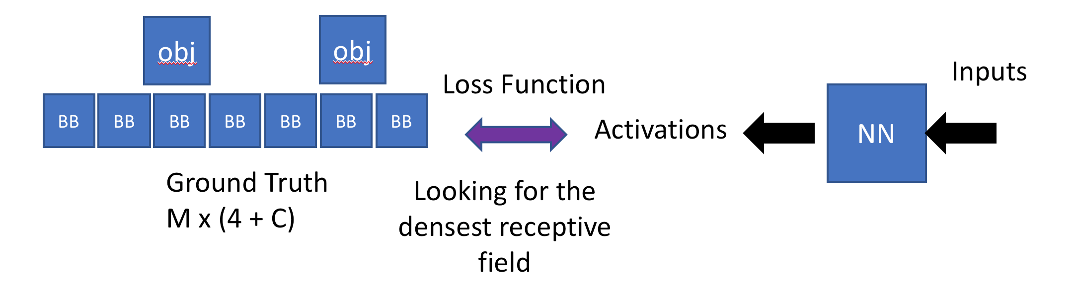
How do we write a loss function for this?
- Has to look at each of these 16 sets of activations, which will each have 4 bounding box and categories + 1
- The loss function actually needs to take each object in the image and match them to a convolutional grid cell. This is called the matching problem
def one_hot_embedding(labels, num_classes):
    return torch.eye(num_classes)[labels.data.cpu()]

class BCE_Loss(nn.Module):
    def __init__(self, num_classes):
        super().__init__()
        self.num_classes = num_classes

    def forward(self, pred, targ):
        t = one_hot_embedding(targ, self.num_classes+1)
        t = V(t[:,:-1].contiguous())#.cpu()
        x = pred[:,:-1]
        w = self.get_weight(x,t)
        return F.binary_cross_entropy_with_logits(x, t, w, size_average=False)/self.num_classes

    def get_weight(self,x,t): return None

loss_f = BCE_Loss(len(id2cat))
Reminder - 4x4 quadrants there’s 20 classes, 1 background + 4 channels
	fn	bbox
0	000012.jpg	96 155 269 350
1	000017.jpg	61 184 198 278 77 89 335 402
Feeds a high number if it IS a good reflection, and a low number is lower.
def intersect(box_a, box_b):
    """ Returns the intersection of two boxes """
    max_xy = torch.min(box_a[:, None, 2:], box_b[None, :, 2:])
    min_xy = torch.max(box_a[:, None, :2], box_b[None, :, :2])
    inter = torch.clamp((max_xy - min_xy), min=0)
    return inter[:, :, 0] * inter[:, :, 1]

def box_sz(b):
    """ Returns the box size"""
    return ((b[:, 2]-b[:, 0]) * (b[:, 3]-b[:, 1]))

def jaccard(box_a, box_b):
    """ Returns the jaccard distance between two boxes"""
    inter = intersect(box_a, box_b)
    union = box_sz(box_a).unsqueeze(1) + box_sz(box_b).unsqueeze(0) - inter
    return inter / union

def get_y(bbox,clas):
    """ ??? """
    bbox = bbox.view(-1,4)/sz
    bb_keep = ((bbox[:,2]-bbox[:,0])>0).nonzero()[:,0]
    return bbox[bb_keep],clas[bb_keep]

def actn_to_bb(actn, anchors):
    """ activations to bounding boxes """
    actn_bbs = torch.tanh(actn)
    actn_centers = (actn_bbs[:,:2]/2 * grid_sizes) + anchors[:,:2]
    actn_hw = (actn_bbs[:,2:]/2+1) * anchors[:,2:]
    return hw2corners(actn_centers, actn_hw)

def map_to_ground_truth(overlaps, print_it=False):
    """ ?? """
    prior_overlap, prior_idx = overlaps.max(1)
    if print_it: print(prior_overlap)
#     pdb.set_trace()
    gt_overlap, gt_idx = overlaps.max(0)
    gt_overlap[prior_idx] = 1.99
    for i,o in enumerate(prior_idx): gt_idx[o] = i
    return gt_overlap,gt_idx

def ssd_1_loss(b_c,b_bb,bbox,clas,print_it=False):
    bbox,clas = get_y(bbox,clas)
    a_ic = actn_to_bb(b_bb, anchors)
    overlaps = jaccard(bbox.data, anchor_cnr.data)
    gt_overlap,gt_idx = map_to_ground_truth(overlaps,print_it)
    gt_clas = clas[gt_idx]
    pos = gt_overlap > 0.4
    pos_idx = torch.nonzero(pos)[:,0]
    gt_clas[1-pos] = len(id2cat)
    gt_bbox = bbox[gt_idx]
    loc_loss = ((a_ic[pos_idx] - gt_bbox[pos_idx]).abs()).mean()
    clas_loss  = loss_f(b_c, gt_clas)
    return loc_loss, clas_loss

def ssd_loss(pred,targ,print_it=False):
    lcs,lls = 0.,0.
    for b_c,b_bb,bbox,clas in zip(*pred,*targ):
        loc_loss,clas_loss = ssd_1_loss(b_c,b_bb,bbox,clas,print_it)
        lls += loc_loss
        lcs += clas_loss
    if print_it: print(f'loc: {lls.data[0]}, clas: {lcs.data[0]}')
    return lls+lcs
Test to make sure that model works
x,y = next(iter(md.val_dl))
#x,y = V(x).cpu(),V(y)
x,y = V(x),V(y)
learn.model.cuda()
batch = learn.model(x)
#ssd_loss(batch, y, True)
learn.model.cuda()
batch = learn.model(x)
type(batch[0].data), type(y[0].data)
(torch.cuda.FloatTensor, torch.cuda.FloatTensor)
Train the model
learn.crit = ssd_loss
lr = 3e-3
lrs = np.array([lr/100,lr/10,lr])

learn.lr_find(lrs/1000,1.)
learn.sched.plot(1)
learn.fit(lr, 1, cycle_len=1, use_clr=(20,3))

learn.fit(lr, 1, cycle_len=5, use_clr=(20,10))
learn.save('0')
epoch      trn_loss   val_loss
    0      178.904678 179954.0


epoch      trn_loss   val_loss
    0      41.900517  30.778248


epoch      trn_loss   val_loss
    0      31.734285  29.830471
    1      29.553838  28.571745
    2      27.744743  26.556757
    3      26.028599  26.084572
    4      24.452854  25.413759
learn.load('0')
Let’s walk through a Loss Function
# grab a single batch
x,y = next(iter(md.val_dl))

# turn into variables
x,y = V(x),V(y)

# set model to eval mode (trained in the previous block)
learn.model.eval()
batch = learn.model(x)

# destructure the class and the bounding box
b_clas,b_bb = batch
The dimensions
- 64 Batch size by
- 16 Grid cells
- 21 classes
- 4 Bounding Box coord
b_clas.size(),b_bb.size()
(torch.Size([64, 16, 21]), torch.Size([64, 16, 4]))
Looking at image 7
idx=7

# class
b_clasi = b_clas[idx]

# bounding box
b_bboxi = b_bb[idx]

# image
ima=md.val_ds.ds.denorm(to_np(x))[idx]

# bounding box / classification
bbox,clas = get_y(y[0][idx], y[1][idx])
bbox,clas
(Variable containing:
  0.6786  0.4866  0.9911  0.6250
  0.7098  0.0848  0.9911  0.5491
  0.5134  0.8304  0.6696  0.9063
 [torch.cuda.FloatTensor of size 3x4 (GPU 0)], Variable containing:
   8
  10
  17
 [torch.cuda.LongTensor of size 3 (GPU 0)])
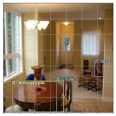
Truth of Image 7
# Convert torch tensors to numpy
def torch_gt(ax, ima, bbox, clas, prs=None, thresh=0.4):
    return show_ground_truth(ax, ima, to_np((bbox*224).long()),
         to_np(clas), to_np(prs) if prs is not None else None, thresh)

fig, ax = plt.subplots(figsize=(7,7))
torch_gt(ax, ima, bbox, clas)
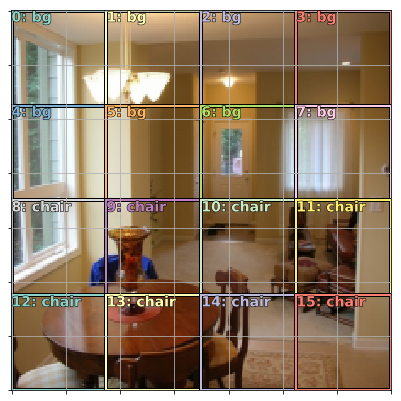
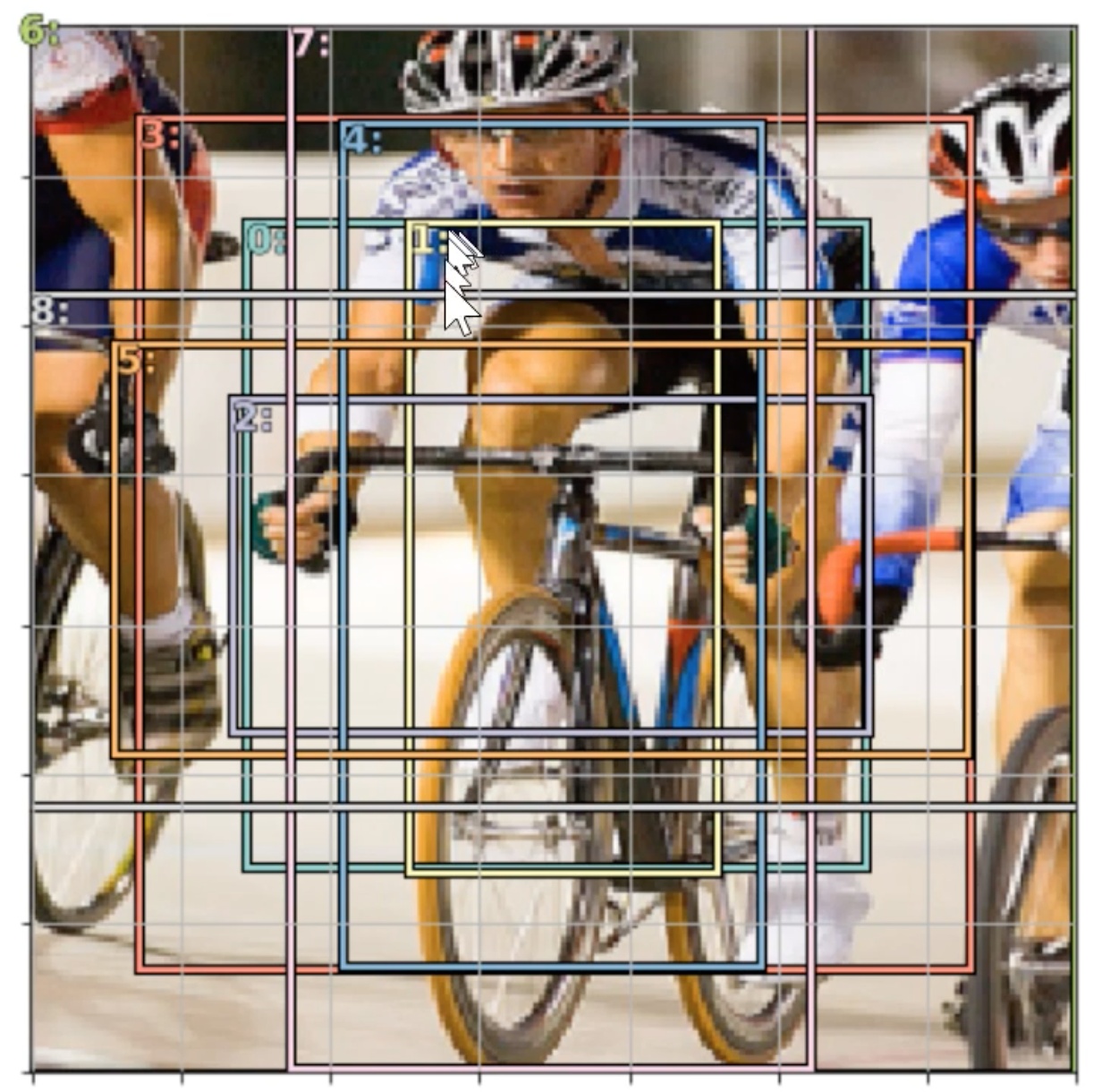
Look at our 16 anchor boxes
fig, ax = plt.subplots(figsize=(7,7))
torch_gt(ax, ima, anchor_cnr, b_clasi.max(1)[1])
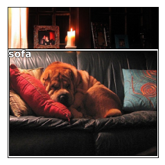
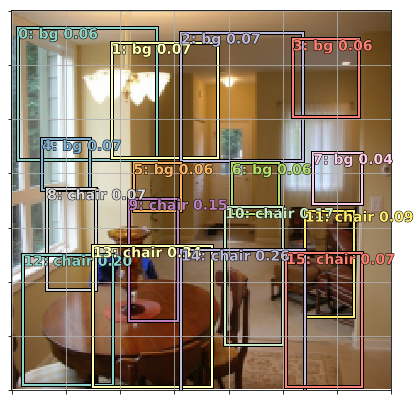
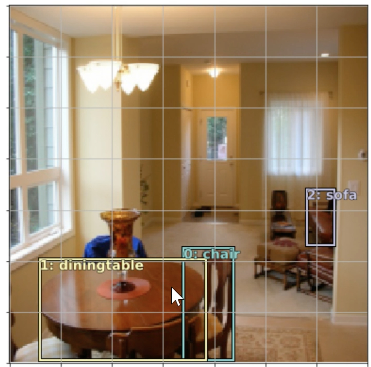
Let’s look at the sofa
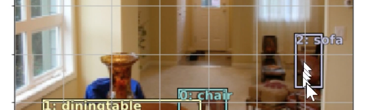
Lets look at the area of intersection with boxes 7 and 11
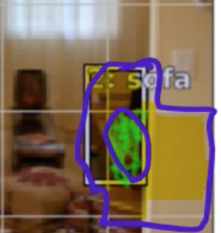
The Jaccard index will be the area of intersection over the area over union. In this picture it is the green area over green + yellow. Higher jaccard index = higher intersection
For Every object ( 0 Chair, 1 Dining, 2 Sofa) we will compare and calc Jaccard index, result is 3x16 matrix
Lets first look at the anchor coordinates. center x | center y | height | width
anchors
Variable containing:
 0.1250  0.1250  0.2500  0.2500
 0.1250  0.3750  0.2500  0.2500
 0.1250  0.6250  0.2500  0.2500
 0.1250  0.8750  0.2500  0.2500
 0.3750  0.1250  0.2500  0.2500
 0.3750  0.3750  0.2500  0.2500
 0.3750  0.6250  0.2500  0.2500
 0.3750  0.8750  0.2500  0.2500
 0.6250  0.1250  0.2500  0.2500
 0.6250  0.3750  0.2500  0.2500
 0.6250  0.6250  0.2500  0.2500
 0.6250  0.8750  0.2500  0.2500
 0.8750  0.1250  0.2500  0.2500
 0.8750  0.3750  0.2500  0.2500
 0.8750  0.6250  0.2500  0.2500
 0.8750  0.8750  0.2500  0.2500
[torch.cuda.FloatTensor of size 16x4 (GPU 0)]
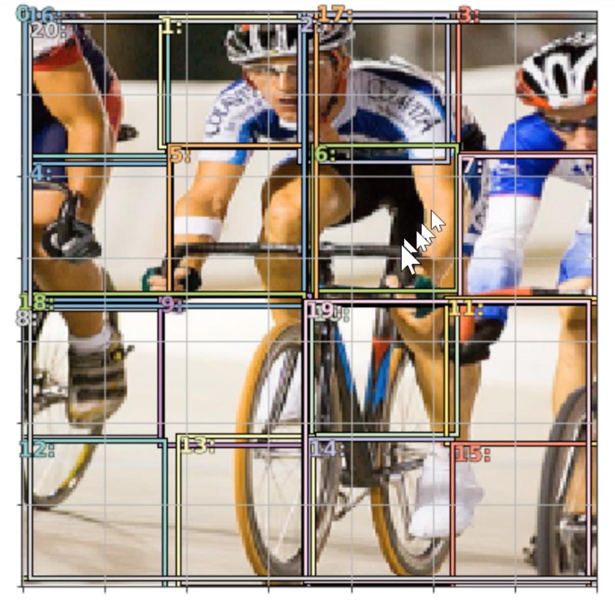
Get the activtions
a_ic = actn_to_bb(b_bboxi, anchors)
fig, ax = plt.subplots(figsize=(7,7))
torch_gt(ax, ima, a_ic, b_clasi.max(1)[1], b_clasi.max(1)[0].sigmoid(), thresh=0.0)
Calculate Jaccard index (all objects x all grid cells)
overlaps = jaccard(bbox.data, anchor_cnr.data)
overlaps
Columns 0 to 9
 0.0000  0.0000  0.0000  0.0000  0.0000  0.0000  0.0000  0.0000  0.0000  0.0091
 0.0000  0.0000  0.0000  0.0000  0.0000  0.0000  0.0000  0.0000  0.0356  0.0549
 0.0000  0.0000  0.0000  0.0000  0.0000  0.0000  0.0000  0.0000  0.0000  0.0000

Columns 10 to 15
 0.0922  0.0000  0.0000  0.0315  0.3985  0.0000
 0.0103  0.0000  0.2598  0.4538  0.0653  0.0000
 0.0000  0.1897  0.0000  0.0000  0.0000  0.0000
[torch.cuda.FloatTensor of size 3x16 (GPU 0)]
For each object, we can find the highest overlap with any cell
Returns:
- Maximum amount
- And the corresponding cell index
# Dining Table
overlaps.max(1)
(
  0.3985
  0.4538
  0.1897
 [torch.cuda.FloatTensor of size 3 (GPU 0)],
  14
  13
  11
 [torch.cuda.LongTensor of size 3 (GPU 0)])
# Chair
overlaps.max(0)
(
  0.0000
  0.0000
  0.0000
  0.0000
  0.0000
  0.0000
  0.0000
  0.0000
  0.0356
  0.0549
  0.0922
  0.1897
  0.2598
  0.4538
  0.3985
  0.0000
 [torch.cuda.FloatTensor of size 16 (GPU 0)],
  0
  0
  0
  0
  0
  0
  0
  0
  1
  1
  0
  2
  1
  1
  0
  0
 [torch.cuda.LongTensor of size 16 (GPU 0)])
Combine overlaps with map_to_ground_truth
- Object gets assigned to a cell if it has maximum value
- Remaining cells get assigned to objects that have 0.5 or more
- All others are considered backgrounds
gt_overlap,gt_idx = map_to_ground_truth(overlaps)
gt_overlap,gt_idx
(
  0.0000
  0.0000
  0.0000
  0.0000
  0.0000
  0.0000
  0.0000
  0.0000
  0.0356
  0.0549
  0.0922
  1.9900
  0.2598
  1.9900
  1.9900
  0.0000
 [torch.cuda.FloatTensor of size 16 (GPU 0)],
  0
  0
  0
  0
  0
  0
  0
  0
  1
  1
  0
  2
  1
  1
  0
  0
 [torch.cuda.LongTensor of size 16 (GPU 0)])
Convert to Classes
gt_clas = clas[gt_idx]; gt_clas
Variable containing:
  8
  8
  8
  8
  8
  8
  8
  8
 10
 10
  8
 17
 10
 10
  8
  8
[torch.cuda.LongTensor of size 16 (GPU 0)]
Comparing Ground Truth Objects to fixed anchor boxes.
thresh = 0.5
pos = gt_overlap > thresh
pos_idx = torch.nonzero(pos)[:,0]
neg_idx = torch.nonzero(1-pos)[:,0]
pos_idx
 11
 13
 14
[torch.cuda.LongTensor of size 3 (GPU 0)]
Show the Cell Assignment
gt_clas[1-pos] = len(id2cat)
[id2cat[o] if o<len(id2cat) else 'bg' for o in gt_clas.data]
['bg',
 'bg',
 'bg',
 'bg',
 'bg',
 'bg',
 'bg',
 'bg',
 'bg',
 'bg',
 'bg',
 'sofa',
 'bg',
 'diningtable',
 'chair',
 'bg']
End the Matching Stage
loc_loss = L1_loss = mean(|matched_activations - ground truth|)
gt_bbox = bbox[gt_idx]
loc_loss = ((a_ic[pos_idx] - gt_bbox[pos_idx]).abs()).mean()
clas_loss  = F.cross_entropy(b_clasi, gt_clas)
loc_loss,clas_loss
(Variable containing:
 1.00000e-02 *
   5.8389
 [torch.cuda.FloatTensor of size 1 (GPU 0)], Variable containing:
  0.8217
 [torch.cuda.FloatTensor of size 1 (GPU 0)])
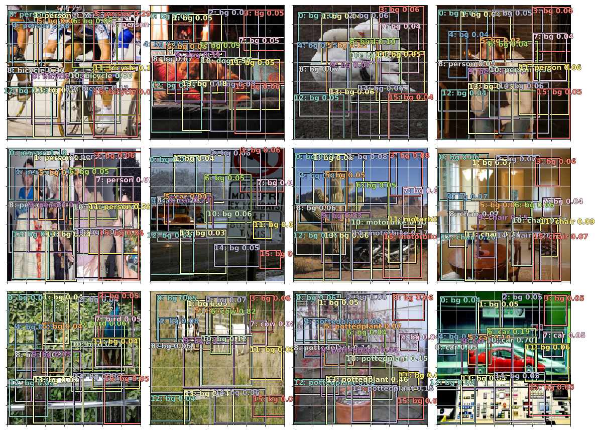
Let’s plot a few pictures
fig, axes = plt.subplots(3, 4, figsize=(16, 12))
for idx,ax in enumerate(axes.flat):
    ima=md.val_ds.ds.denorm(to_np(x))[idx]
    bbox,clas = get_y(y[0][idx], y[1][idx])
    ima=md.val_ds.ds.denorm(to_np(x))[idx]
    bbox,clas = get_y(bbox,clas); bbox,clas
    a_ic = actn_to_bb(b_bb[idx], anchors)
    torch_gt(ax, ima, a_ic, b_clas[idx].max(1)[1], b_clas[idx].max(1)[0].sigmoid(), 0.01)
plt.tight_layout()
Clipping input data to the valid range for imshow with RGB data ([0..1] for floats or [0..255] for integers).
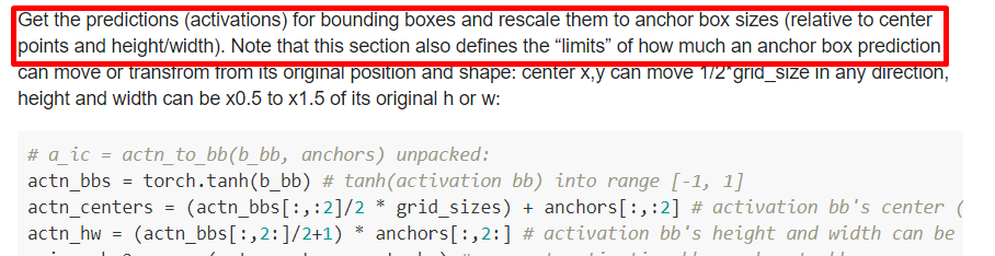
How do we interpret Activations?
Each predicted bounding box, can be moved up to 50%, twice or half as large. We have to convert the activations into a scaling.
def actn_to_bb(actn, anchors):
    """ activations to bounding boxes """
    actn_bbs = torch.tanh(actn)
    actn_centers = (actn_bbs[:,:2]/2 * grid_sizes) + anchors[:,:2]
    actn_hw = (actn_bbs[:,2:]/2+1) * anchors[:,2:]
    return hw2corners(actn_centers, actn_hw)
Each box can only have one object associated with it. Its possible for an anchorbox to have NOTHING in it. We could:
- treat background as a class - difficult, because its asking the NN to say ‘does this square NOT have 20 other things’
- BCE loss, checks by process of elimination - if there’s no 20 objecst detected, then its background (0 positives)
def one_hot_embedding(labels, num_classes):
    return torch.eye(num_classes)[labels.data.cpu()]

class BCE_Loss(nn.Module):
    def __init__(self, num_classes):
        super().__init__()
        self.num_classes = num_classes

    def forward(self, pred, targ):
        t = one_hot_embedding(targ, self.num_classes+1)
        t = V(t[:,:-1].contiguous())#.cpu()
        x = pred[:,:-1]
        w = self.get_weight(x,t)
        return F.binary_cross_entropy_with_logits(x, t, w, size_average=False)/self.num_classes

    def get_weight(self,x,t): return None

loss_f = BCE_Loss(len(id2cat))
SSD Loss
# total SSD loss for batch
def ssd_loss(pred,targ,print_it=False):
    lcs,lls = 0.,0.
    for b_c,b_bb,bbox,clas in zip(*pred,*targ):
        loc_loss,clas_loss = ssd_1_loss(b_c,b_bb,bbox,clas,print_it)
        lls += loc_loss
        lcs += clas_loss
    if print_it: print(f'loc: {lls.data[0]}, clas: {lcs.data[0]}')
    return lls+lcs

# SSD loss for one image
def ssd_1_loss(b_c,b_bb,bbox,clas,print_it=False):

    # get bounding box and classes
    bbox,clas = get_y(bbox,clas)

    # activations to bounding box
    a_ic = actn_to_bb(b_bb, anchors)

    # calculate overlaps
    overlaps = jaccard(bbox.data, anchor_cnr.data)

    # get the overlaps based on the criteria
    gt_overlap,gt_idx = map_to_ground_truth(overlaps,print_it)

    # get the classes
    gt_clas = clas[gt_idx]

    # find the positives
    pos = gt_overlap > 0.4
    pos_idx = torch.nonzero(pos)[:,0]

    # do the cell assignments
    gt_clas[1-pos] = len(id2cat)
    gt_bbox = bbox[gt_idx]

    # calc L1 loss and cross entropy loss
    loc_loss = ((a_ic[pos_idx] - gt_bbox[pos_idx]).abs()).mean()
    clas_loss  = loss_f(b_c, gt_clas)
    return loc_loss, clas_loss
How can we improve?
Let’s increase the resolution of the anchor boxes.
Create Anchor Boxes of different sizes / Aspect Ratios ( 3 aspect ratios, 3 zooms)
Use more conv. layers as source of anchor boxes
4 x 4 , 2 x 2, 1 x 1
We can combine the methods to create a LOT of anchor boxes
# Grid cell sizes
anc_grids = [4,2,1]
anc_zooms = [0.75, 1., 1.3]
anc_ratios = [(1.,1.), (1.,0.5), (0.5,1.)]
anchor_scales = [(anz*i,anz*j) for anz in anc_zooms for (i,j) in anc_ratios]
k = len(anchor_scales)
anc_offsets = [1/(o*2) for o in anc_grids]
k
9
Make the Corners
anc_x = np.concatenate([np.repeat(np.linspace(ao, 1-ao, ag), ag)
                        for ao,ag in zip(anc_offsets,anc_grids)])
anc_y = np.concatenate([np.tile(np.linspace(ao, 1-ao, ag), ag)
                        for ao,ag in zip(anc_offsets,anc_grids)])
anc_ctrs = np.repeat(np.stack([anc_x,anc_y], axis=1), k, axis=0)
Make the Dimensions
anc_sizes  =   np.concatenate([np.array([[o/ag,p/ag] for i in range(ag*ag) for o,p in anchor_scales])
               for ag in anc_grids])
grid_sizes = V(np.concatenate([np.array([ 1/ag       for i in range(ag*ag) for o,p in anchor_scales])
               for ag in anc_grids]), requires_grad=False).unsqueeze(1)
anchors = V(np.concatenate([anc_ctrs, anc_sizes], axis=1), requires_grad=False).float()
anchor_cnr = hw2corners(anchors[:,:2], anchors[:,2:])
Change our Architecture, so it spits out enough activations, Sample of Ground Truth
Try to make the activations who closely represents the bounding box
- Now we can have multiple anchor boxes per grid cell
- For every object, have to figure out which anchor box which is closer
- For each anchor box, we have to find which object its responsible for
- We don’t need to necessarily change the number of Conv. Filters. We will get these for free
For ground truth boxes = n x (4 + c)
here’s the Model
-
k= number of zooms x number of aspect ratios. Grids will be for free -
Note the number of
OutConvthere’s many more outputs this time around
class SSD_MultiHead(nn.Module):
    def __init__(self, k, bias, drop=0.1):
        super().__init__()
        self.drop = nn.Dropout(drop)
        self.sconv1 = StdConv(512,256, drop=drop)
        self.sconv2 = StdConv(256,256, drop=drop)
        self.sconv3 = StdConv(256,256, drop=drop)
        self.out0 = OutConv(k, 256, bias)
        self.out1 = OutConv(k, 256, bias)
        self.out2 = OutConv(k, 256, bias)
        self.out3 = OutConv(k, 256, bias)

    def forward(self, x):
        x = self.drop(F.relu(x))
        x = self.sconv1(x)
        o1c,o1l = self.out1(x)
        x = self.sconv2(x)
        o2c,o2l = self.out2(x)
        x = self.sconv3(x)
        o3c,o3l = self.out3(x)
        return [torch.cat([o1c,o2c,o3c], dim=1),
                torch.cat([o1l,o2l,o3l], dim=1)]

head_reg4 = SSD_MultiHead(k, -4.)
models = ConvnetBuilder(f_model, 0, 0, 0, custom_head=head_reg4)
learn = ConvLearner(md, models)
learn.opt_fn = optim.Adam
learn.crit = ssd_loss
lr = 1e-2
lrs = np.array([lr/100,lr/10,lr])
learn.lr_find(lrs/1000,1.)
learn.sched.plot(n_skip_end=2)
epoch      trn_loss   val_loss
    0      436.807953 900833.375
learn.fit(lrs, 1, cycle_len=4, use_clr=(20,8))
epoch      trn_loss   val_loss
    0      153.950207 126.174835
    1      119.084206 96.903702
    2      99.650275  86.885757
    3      86.064523  81.786957


[81.78696]
learn.save('tmp')
learn.freeze_to(-2)
learn.fit(lrs/2, 1, cycle_len=4, use_clr=(20,8))
epoch      trn_loss   val_loss
    0      81.888921  154.412491
    1      77.393581  86.504921
    2      69.236292  77.665382
    3      61.646758  74.613998


[74.614]
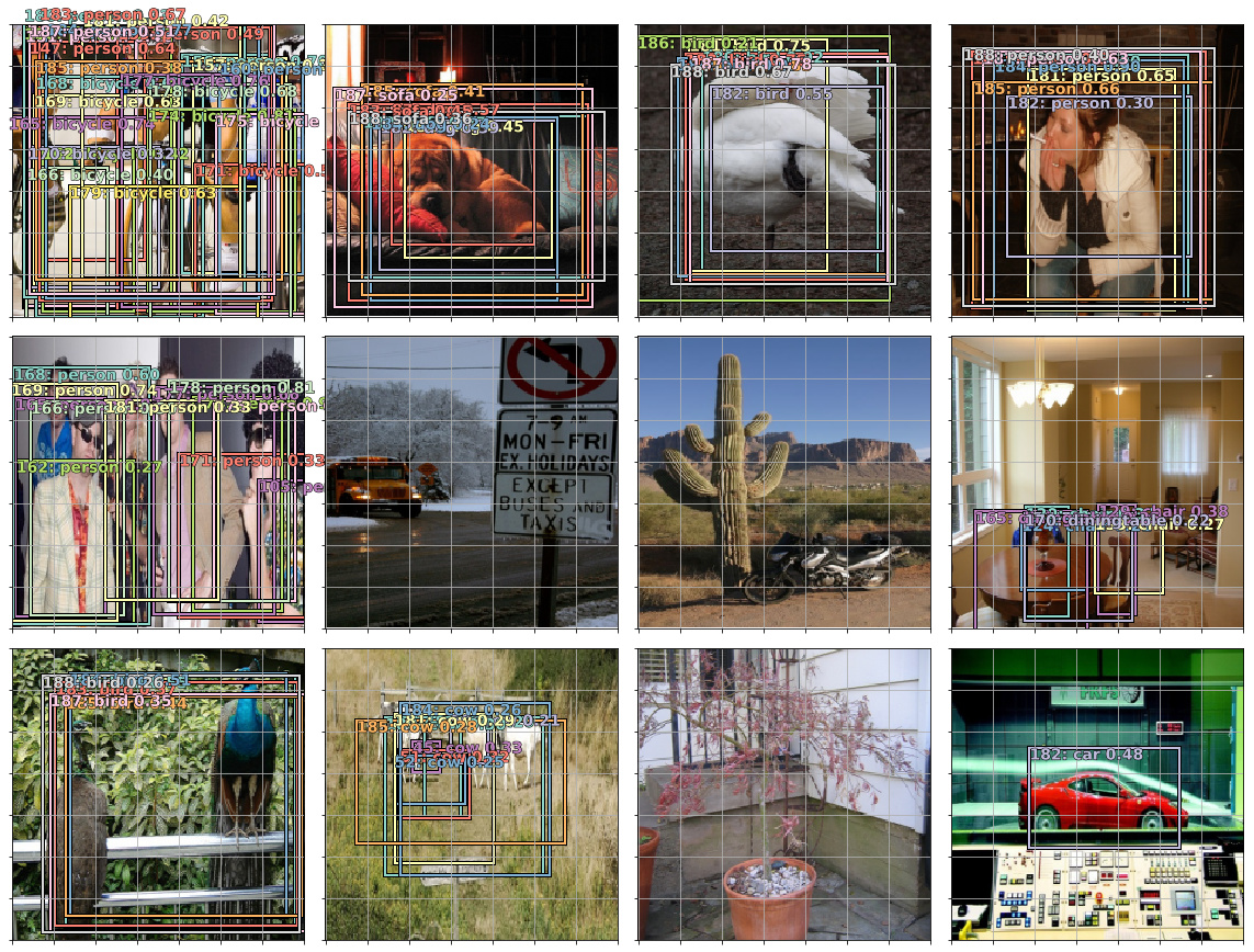
Lets look at a batch with probability 0.1
x,y = next(iter(md.val_dl))
y = V(y)
batch = learn.model(V(x))
b_clas,b_bb = batch
x = to_np(x)

fig, axes = plt.subplots(3, 4, figsize=(16, 12))
for idx,ax in enumerate(axes.flat):
    ima=md.val_ds.ds.denorm(x)[idx]
    bbox,clas = get_y(y[0][idx], y[1][idx])
    a_ic = actn_to_bb(b_bb[idx], anchors)
    torch_gt(ax, ima, a_ic, b_clas[idx].max(1)[1], b_clas[idx].max(1)[0].sigmoid(), 0.2)
plt.tight_layout()
Clipping input data to the valid range for imshow with RGB data ([0..1] for floats or [0..255] for integers).
Rich History of Object Detection
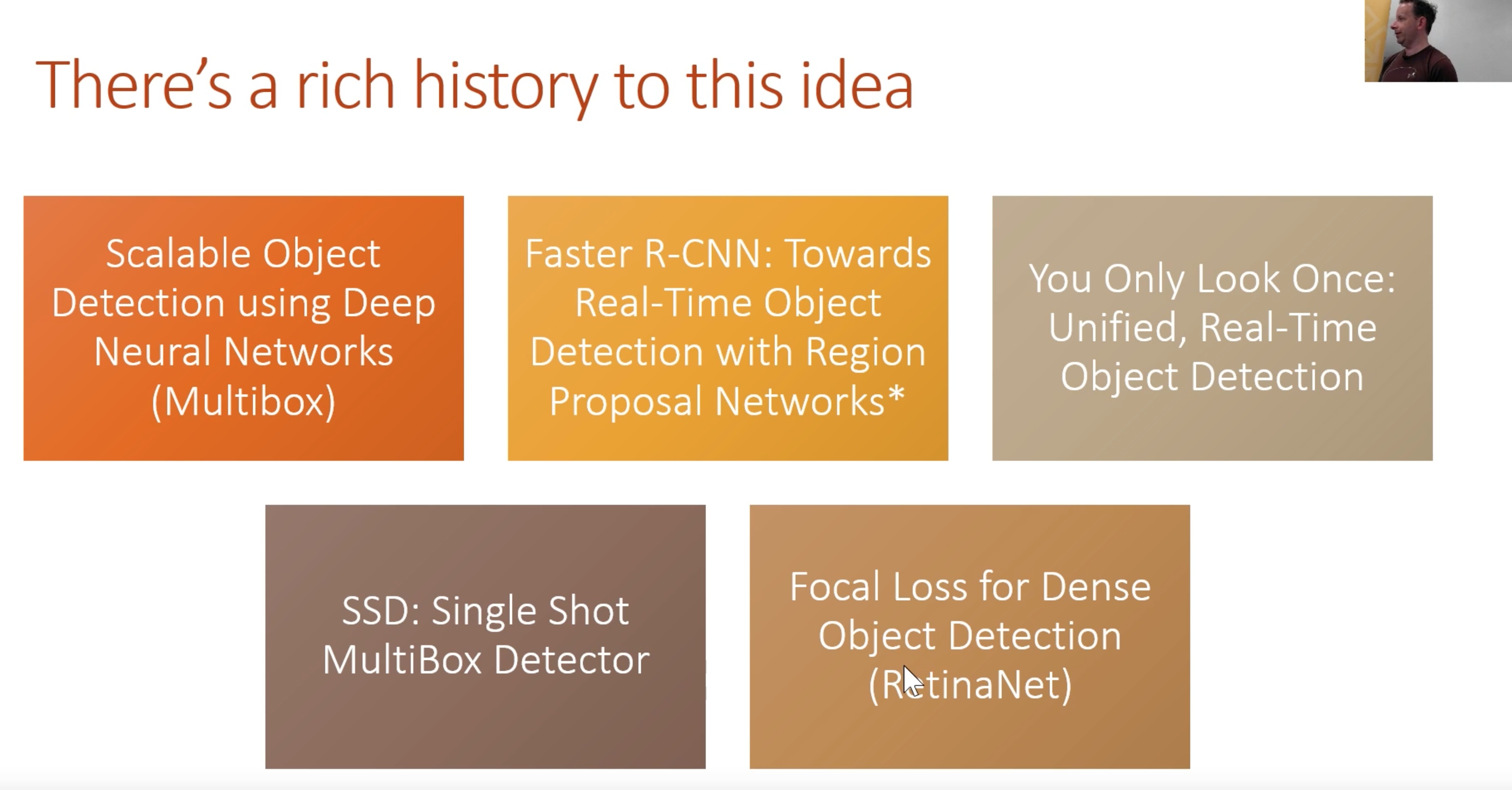
- 2013 - Multibox method paper. You can have a loss function with a matching process
- Ross Girshick - one conv net makes region proposals, one conv net, fed each region into a separate classifier FAST RCNN
- YOLO & SSD - multibox, but cut through the clutter
- 2017 - FOCAL LOSS RetinaNet - the messy crap doesn’t work.
Where’s the bike!?
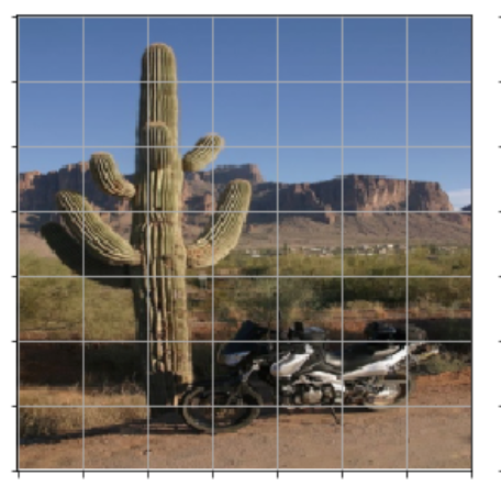
If you have a 1 x 1, there’s a good chance you will find an image. If you have a 4 x 4 search, there’s a reduced chance that an object.
Why overlapping + large numbers of anchor boxes?
The jacarrad index calculation makes it difficult to achieve over 0.5 without different sized boxes.
Consider reading the paper.
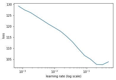
Paper
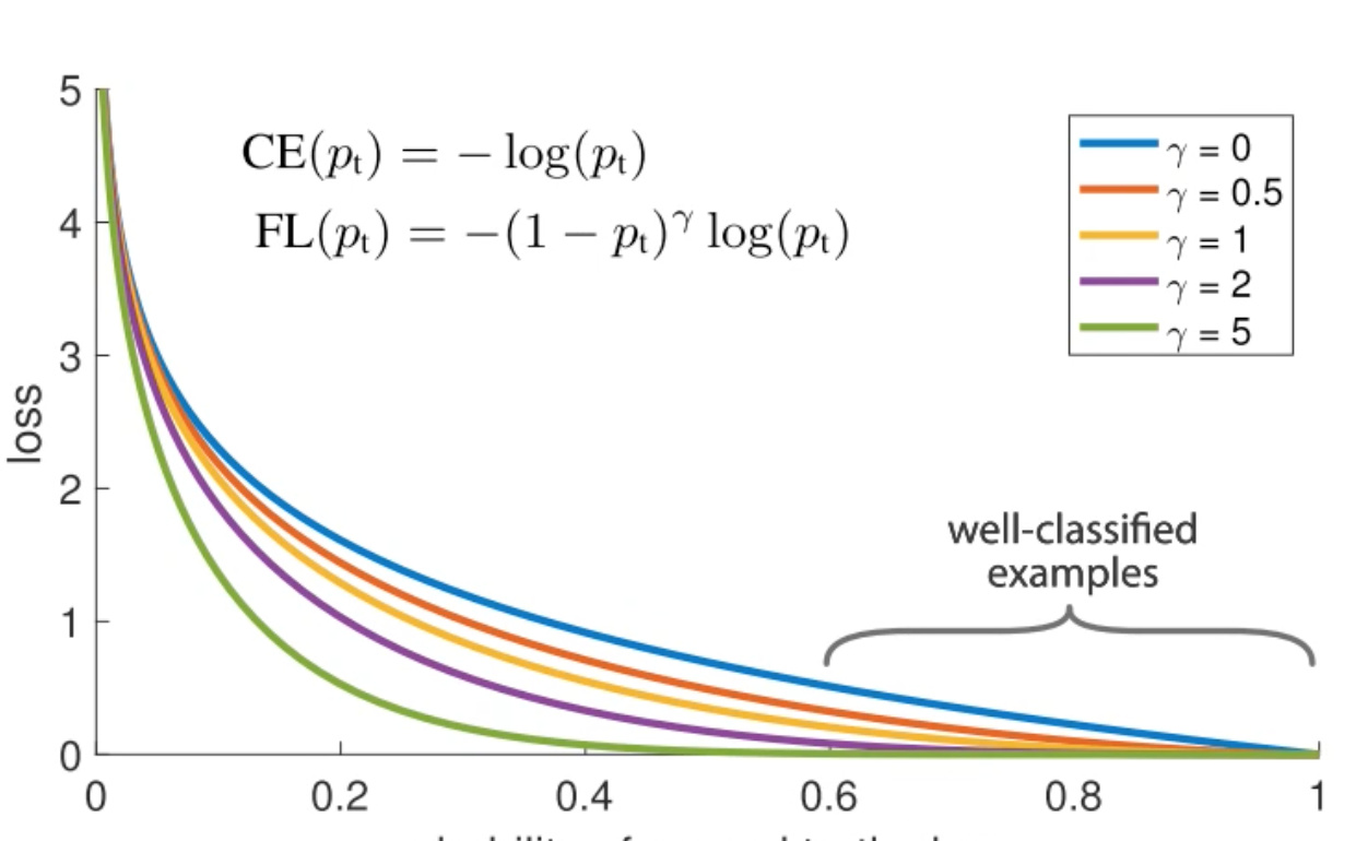
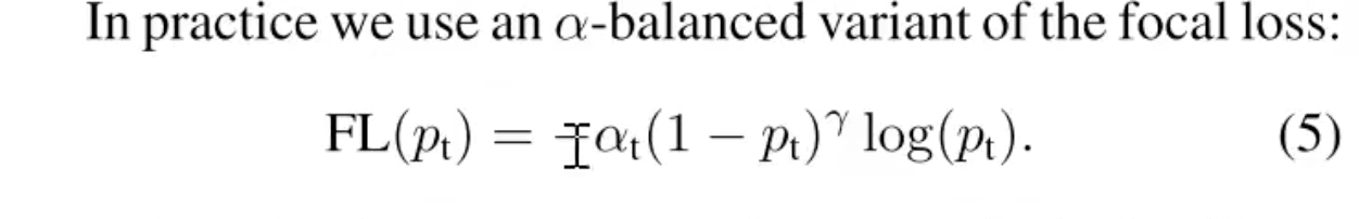
Considering the blue line, even if we are at 0.6 confident, the loss is still pretty high. You can’t simply say its “not background” you have to be confident its one of the 20 classes. So for smaller objects, its not confident enough. Thats also why the boxes are so big for some objects.
So they suggest a new loss function - purple line. The FL function is a scaling function of cross entropy loss
It is amazing that the solution is very elegant, and very straightforward in execution.

How to deal with Class imbalance
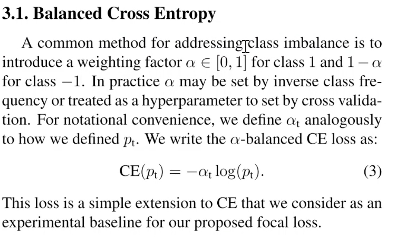
Then they define Focal Loss with Class weighting
Focal Loss
def plot_results(thresh):
    x,y = next(iter(md.val_dl))
    y = V(y)
    batch = learn.model(V(x))
    b_clas,b_bb = batch

    x = to_np(x)
    fig, axes = plt.subplots(3, 4, figsize=(16, 12))
    for idx,ax in enumerate(axes.flat):
        ima=md.val_ds.ds.denorm(x)[idx]
        bbox,clas = get_y(y[0][idx], y[1][idx])
        a_ic = actn_to_bb(b_bb[idx], anchors)
        clas_pr, clas_ids = b_clas[idx].max(1)
        clas_pr = clas_pr.sigmoid()
        torch_gt(ax, ima, a_ic, clas_ids, clas_pr, clas_pr.max().data[0]*thresh)
    plt.tight_layout()
class FocalLoss(BCE_Loss):
    def get_weight(self,x,t):
        alpha,gamma = 0.25,2.
        p = x.sigmoid()
        pt = p*t + (1-p)*(1-t)
        w = alpha*t + (1-alpha)*(1-t)
        return w * (1-pt).pow(gamma)

loss_f = FocalLoss(len(id2cat))
Retrain the model
learn.lr_find(lrs/1000,1.)
learn.sched.plot(n_skip_end=2)
91%|█████████ | 29/32 [00:18<00:01, 1.53it/s, loss=53.9]
learn.fit(lrs, 1, cycle_len=10, use_clr=(20,10))
  0%|          | 0/32 [00:00<?, ?it/s]


Exception in thread Thread-57:
Traceback (most recent call last):
  File "/home/paperspace/anaconda3/envs/fastai/lib/python3.6/threading.py", line 916, in _bootstrap_inner
    self.run()
  File "/home/paperspace/anaconda3/envs/fastai/lib/python3.6/site-packages/tqdm/_tqdm.py", line 144, in run
    for instance in self.tqdm_cls._instances:
  File "/home/paperspace/anaconda3/envs/fastai/lib/python3.6/_weakrefset.py", line 60, in __iter__
    for itemref in self.data:
RuntimeError: Set changed size during iteration


epoch      trn_loss   val_loss
    0      14.627009  27.391459
    1      17.046875  55.384224
    2      15.914187  15.103384
    3      14.135144  13.905497
    4      12.67438   12.506262
    5      11.445519  13.349274
    6      10.465744  11.700116
    7      9.644463   11.588182
    8      8.954488   11.204657
    9      8.42627    11.142858


[11.142858]
learn.save('fl0')
learn.load('fl0')
learn.freeze_to(-2)
learn.fit(lrs/4, 1, cycle_len=10, use_clr=(20,10))
epoch      trn_loss   val_loss
    0      7.77895    11.484667
    1      7.945573   11.758629
    2      7.907224   11.412073
    3      7.673045   11.21604
    4      7.334933   11.071276
    5      7.017753   11.007197
    6      6.75496    11.007086
    7      6.531224   10.968062
    8      6.319731   10.930752
    9      6.154025   10.955283


[10.955283]
learn.save('drop4')
learn.load('drop4')
x,y = next(iter(md.val_dl))
x,y = V(x),V(y)
batch = learn.model(x)
#ssd_loss(batch, y, True)
plot_results(0.75)
Clipping input data to the valid range for imshow with RGB data ([0..1] for floats or [0..255] for integers).
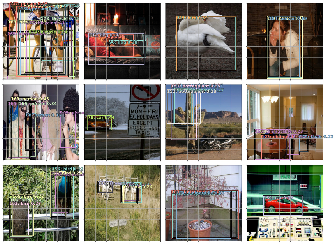
Non-Maximum Suppression
- Will review the different boxes and compares if the boxes overlap a lot, and if they predict the same thing, and will eliminate the duplicate with the lower p-value.
 That’s all the comments I have.