Part 2 Lesson 9 wiki

radek · April 5, 2018, 2:14pm

I think you are on the right track.

Softmax output with cross entropy cost => one question, which out of the n classes does this object belong to? probabilities sum to 1

n sigmoid outputs with binary cross entropy cost => n questions, is this object of class 0? is this object of class 1? etc Can be used with multiple labels and also we no longer have to ask our NN to identify background, which the idea is that it might be easier to do for the NN then learning a whole new class for ‘there is nothing here’

alwc · April 5, 2018, 4:58pm

Logistic function (sigmoid function is a special case of logistic function) and softmax function can be defined as “score functions”. They output real value(s) in the range (0, 1).
Logistic function assumed that the labels were binary. Softmax function is the generalization of the logistic function that allows us to handle K classes instead.
Logistic loss (a.k.a. binary cross-entropy loss) and (categorical) cross-entropy loss are loss functions. It uses to find the difference between the prediction versus the ground-truth label.

For example, for binary logistic regression with ground truth label \mathbf{y} \in \mathbb{R}^2, we use logistic function + binary cross-entropy (BCE) loss:

\mathbf{z} = \mathbf{Wx + b} \\ \hat{\mathbf{y}} = \text{logistic}(\mathbf{z}) \in \mathbb{R}^2 \\ \mathcal{L}_{\text{BCE}}(\mathbf{y}, \mathbf{\hat{y}}) = - \sum_{k=1}^2 y_k \log \hat{y}_k \in \mathbb{R}

For multinomial logistic regression (a.k.a. softmax regression) with ground truth label \mathbf{y} \in \mathbb{R}^K, we use softmax function + (categorical) cross-entropy (CE) loss:

\mathbf{z} = \mathbf{Wx + b} \\ \hat{\mathbf{y}} = \text{softmax}(\mathbf{z}) \in \mathbb{R}^K \\ \mathcal{L}_{\text{CE}}(\mathbf{y}, \mathbf{\hat{y}}) = -\sum_{k=1}^{K} y_k \log \hat{y}_k = - \mathbf{y}^T \log \hat{\mathbf{y}} \in \mathbb{R}

Note that \mathbf{y} is an one-hot encoded ground-truth vector.

chunduri · April 5, 2018, 5:28pm

hi @radek my understanding is that, in an image, we have multiple objects to be detected.

Each object in the image is a multi-class classification problem, so the obvious choice should be to use softmax for each object and then use cross-entropy to calculate the loss.

“n sigmoid outputs with binary cross entropy cost =>”, so why do u make this statement. Is there a role for sigmoid function and binary cross entropy in this multi-object multi-class detection?

There must be something obvious here but i am not getting the intuition behind using n sigmoids.

I am trying to clarify my fundamental discomfort with loss calculation.

radek · April 5, 2018, 7:34pm

It is all about how you frame the question. Lets consider a single anchor box where we want to classify if it belongs to one of the categories (person, bottle, etc). If we have 20 classes, we can ask our NN 20 questions - is this a person? is this a bottle? is this a table? etc. If the network answers no to all these questions (probability of class below certain threshold value), then this implies that we are looking at an anchor box of class bg. But we never asked our NN to learn to predict the background class!

Alternatively, we could have 21 outputs (20 classes + 1 extra class for bg) and ask a question using softmax - which is the class associated with this anchor box? Asking this question would require our NN to learn to predict the bg class! This, as far as I understand, is considered a harder question to ask. I have not gotten to the point where I have played with this (I will!) but I would guess that people ran experiments and using sigmoid activations with binary cross entropy loss turned out to work better.

radek · April 6, 2018, 9:34am

download

Why do we divide by 2 here? If I understand correctly, we are doing this to limit the offsets to max 0.5 the width / height of the grid cell?

alwc · April 6, 2018, 11:27am

davidluo has written down a step-by-step guide of SSD loss that you may be interested of it.

According to his note:

# activation bb's center (x,y) can be up to 1/2*grid_sizes offset from original anchor box center
actn_centers = (actn_bbs[:,:2]/2 * grid_sizes) + anchors[:,:2] 

# activation bb's height and width can be between 0.5-1.5x the original anchor box h&w
actn_hw = (actn_bbs[:,2:]/2+1) * anchors[:,2:]

alessa · April 6, 2018, 5:31pm

Each predicted BoundedBox can be moved by 50% of a grid size from where its default position is, and the size can be up to twice as big If it makes sense

Chris_Palmer · April 8, 2018, 1:24pm

Confused about my results, and looking for guidance.

My big difference is that I am forced to use a batch size of 32 because of my old GPU.

My results are all over the place when compared with Jeremy’s.

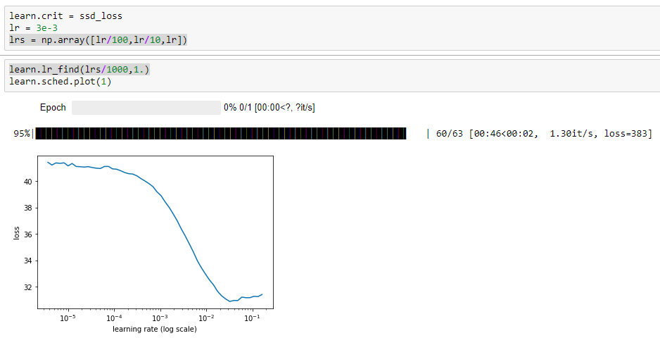
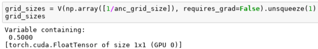
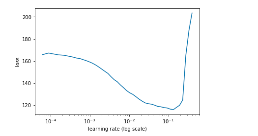
For instance after the initial learn.model() and the application of lr = 3e-3, lrs = np.array([lr/100,lr/10,lr]), learn.lr_find(lrs/1000,1.)

My plot:

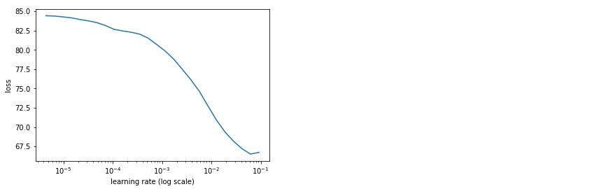
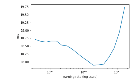
Jeremy’s plot:

Then after learn.fit(lr, 1, cycle_len=5, use_clr=(20,10))

My results:

epoch      trn_loss   val_loss                                                                                         
    0      19.368023  15.716943 
    1      15.620254  14.04254                                                                                         
    2      13.78509   13.574283                                                                                        
    3      12.395073  13.149381                                                                                        
    4      11.260969  12.904029                                                                                        

[12.904029130935669]

Jeremy’s:

epoch      trn_loss   val_loss                            
    0      43.166077  32.56049  
    1      33.731625  28.329123                           
    2      29.498006  27.387726                           
    3      26.590789  26.043869                           
    4      24.470896  25.746592                           

[25.746592]

Well, this looks good at this stage, but why is everything roughly half / twice?

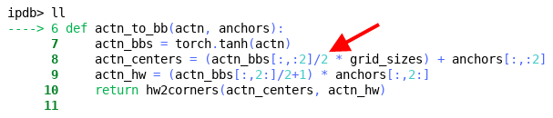
But after all of the next process of testing, creating more anchors, then the Model section we come to:

learn.crit = ssd_loss
lr = 1e-2
lrs = np.array([lr/100,lr/10,lr])
x,y = next(iter(md.val_dl))
x,y = V(x),V(y)
batch = learn.model(V(x))

batch[0].size(),batch[1].size()
(torch.Size([32, 189, 21]), torch.Size([32, 189, 4]))

ssd_loss(batch, y, True)

I end up with this:

Variable containing:
 164.1034
[torch.cuda.FloatTensor of size 1 (GPU 0)]

Jeremy has:

Variable containing:
 4.5301
[torch.cuda.FloatTensor of size 1 (GPU 0)]
 Variable containing:
 61.3364
[torch.cuda.FloatTensor of size 1 (GPU 0)]

Variable containing:
 65.8664
[torch.cuda.FloatTensor of size 1 (GPU 0)]

Only one Variable in my notebook?

After learn.lr_find(lrs/1000,1.), learn.sched.plot(n_skip_end=2), and plot I have:

Jeremy has:

With learn.fit(lrs, 1, cycle_len=4, use_clr=(20,8)) I have:

epoch      trn_loss   val_loss                                                                                         
    0      72.285796  57.328072 
    1      57.207861  48.549717                                                                                        
    2      48.630814  44.12774                                                                                         
    3      43.100264  41.231654

Jeremy has:

epoch      trn_loss   val_loss                            
    0      23.020269  22.007149 
    1      19.23732   15.323267                           
    2      16.612079  13.967303                           
    3      14.706582  12.920008                           

[12.920008]

After that I do my best at adjusting the lr (and subsequent lrs) and use_clr
e.g. tried lr = 1e-3, tried use_clr=(60,10) and got this upon retesting lr:

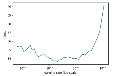
But the best I’ve achieved is this and I’m just spinning my wheels:

epoch      trn_loss   val_loss                                                                                         
    0      33.419068  39.042112 
    1      32.294365  38.817078                                                                                        
    2      31.792605  38.655365                                                                                        
    3      31.260753  38.581855

ANY ADVICE ANYONE?

jeremy · April 8, 2018, 2:51pm

That all looks fine. I don’t run my notebook in order so you shouldn’t expect the same results. Losses depend on # anchors so you and I likely used different numbers.

Focus on the pictures! See if your bounding boxes and classifications look reasonable.

Chris_Palmer · April 8, 2018, 5:02pm

OK, thanks Jeremy. I will carry on - I used these combinations for anchors:

anc_grids = [4,2,1]
anc_zooms = [0.7, 1., 1.3]
anc_ratios = [(1.,1.), (1.,0.5), (0.5,1.)]

Can you please explain the difference in Variable count at the end of running ssd_loss?

It seemed amazing to me that I could start and finish at such a high error rate compared with you, and I experimented with increasing the first parameter of use_clr as there was so much more difference between the points on my learning rate graph - not sure if I have understood that properly…

UPDATE:
I carried on, and got as far as displaying bounding boxes in the code section just after learn.save('prefocal') - the result below. Unfortunately the next time I ran the learning rate finder my GPU crashed. I know it’s way past time I upgraded from a 2GB GPU - its not worth the time and effort to juggle with these tiny resources

chunduri · April 9, 2018, 6:53am

your explanation clubbed with the diagram you provided in the forums and also shown in the class, has cleared all my confusion about, how anchor boxes are selected from the last few convolution layers. And also the difference between “sconv” and “oconv”, is clear now.

thankyou

alessiamarcolini · April 11, 2018, 9:20pm

Batch norm has to be after a relu and not before

alessiamarcolini · April 11, 2018, 9:24pm

Usually values from 0.2 to 0.5 work well

visingh · April 13, 2018, 6:19pm

Not sure, if anyone else faced this error, with show_ground_truth function. Basically the data loader is appending 0’s in front of bboxes to make them all of equal length. when passed such a bbox (zero appended) the bb_hw function converts that to a rect of (0,0,1,1) and when you go plotting this bbox, you get following:

We are getting aeroplane i.e. cat2id[0], foe every image in top left corner because that’s how clas list also hass some zero’s appended in front of it as passed by the data loader.

tagging @jeremy in this as i think this is happening in latest form of notebooks.

visingh · April 13, 2018, 6:21pm

I fixed this by changing the show_ground_truth to following

and the plots seem ok now

radek · April 15, 2018, 6:42am

For the anchor box that overlaps most with gt, we set its IOU to 1.99.

download

Q1. Is there a reason for the choice of this value?

My understanding is that it could be anything big enough and I suppose we might have gone with 1.99 cause it stands quite a bit out from values we expect to be floats < 1, but I wonder if maybe there is anything else to this that I am missing.

Q2. Is the intent of the code below to show non max suppressed results of our model?

Q3. Please verify my understanding if you were so kind please

The below image depicts non max suppressed results. Initially, I thought it is incorrect - the smaller box is fully contained inside the bigger one so it should be suppressed. Then I realized - NMS will only suppress the less confident in its results prediction if its overlap with the other one ise > threshold. Meaning - if there will be an adequately small box inside a big box, the small box will not get suppressed. This is by design - if boxes are that much apart in sizes, the idea is that they might be predicting different objects and we do not wan to get rid of either of them.

download

jeremy · April 15, 2018, 2:15pm

Nothing else - that’s the whole reason.

Yes that’s the idea.

rohitgeo · April 15, 2018, 6:13pm

I also ran into another reason why md.val_ds and val_mcs might not to line up - if the CSV file does not have the filenames in a sorted order. ImageClassifierData.from_csv sorts them while creating the training and validation sets. If we don’t sort the trn_ids similarly, they won’t line up correctly in the ConcatLblDataset…

radek · April 16, 2018, 8:27am

I am probably missing something obvious here.

download

We use grid_sizes in the calculations to go from the activations to the predictions. So the gradient has to flow through them so that we can backpropagate the error. But this is essentially a constant. Why does it have to be a variable? Does it have to be a variable?

If I change grid_sizes to be a FloatTensor I get the error above. So seems it either wants a float or a Variable… mhmmm.

I realize that this will change in PyTorch 0.4, but could this be that gradients just cannot float through tensors that are not Variables?

I now tried running the code with grid_sizes being just a Python float and it works. So this seems like a limitation of PyTorch tensors that they can’t be used as constants? You either need a Variable or some numeric value as plain Tensors cannot be part of the computational graph as they lack some necessary functionality?

Edit: But we cannot keep the grid_sizes as a Python float since down the road we want different sizes of anchors per each grid cell… so if I am reading this right, because we cannot use floats in our situation, np.arrays cannot be part of the computational graph… Tensors are of limits cause they don’t allow the flow of gradients through them… we need to use Variables?

jeremy · April 16, 2018, 1:41pm

That’s basically right. The exact problem is that there are no ‘rank 0 tensors’ in pytorch. So scalars are considered ‘special’ - in the way you see above, amongst others. Really this should be a rank-0 variable, but that doesn’t exist.

Pytorch 0.4, I believe, will introduce rank 0 tensors. (And will get rid of variables, perhaps.)