your explanation clubbed with the diagram you provided in the forums and also shown in the class, has cleared all my confusion about, how anchor boxes are selected from the last few convolution layers. And also the difference between “sconv” and “oconv”, is clear now.
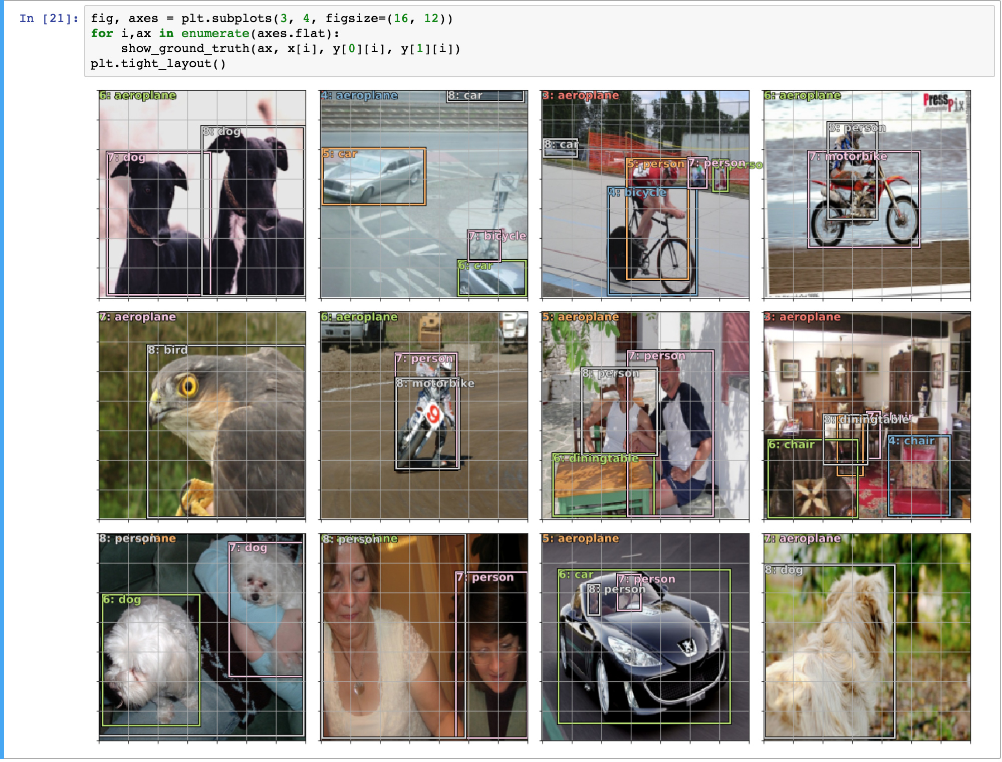
Not sure, if anyone else faced this error, with show_ground_truth function. Basically the data loader is appending 0’s in front of bboxes to make them all of equal length. when passed such a bbox (zero appended) the bb_hw function converts that to a rect of (0,0,1,1) and when you go plotting this bbox, you get following:
We are getting aeroplane i.e. cat2id[0], foe every image in top left corner because that’s how clas list also hass some zero’s appended in front of it as passed by the data loader.
tagging @jeremy in this as i think this is happening in latest form of notebooks.
For the anchor box that overlaps most with gt, we set its IOU to 1.99.
Q1. Is there a reason for the choice of this value?
My understanding is that it could be anything big enough and I suppose we might have gone with 1.99 cause it stands quite a bit out from values we expect to be floats < 1, but I wonder if maybe there is anything else to this that I am missing.
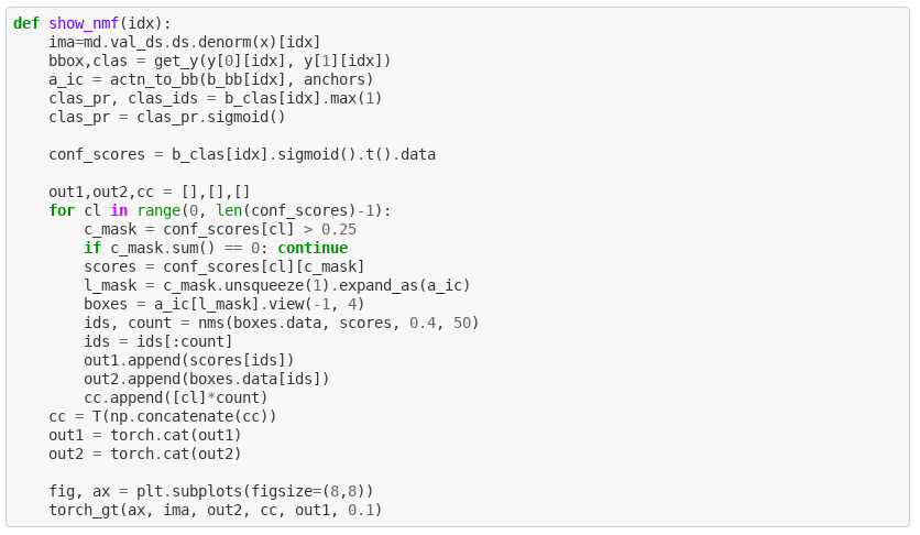
Q2. Is the intent of the code below to show non max suppressed results of our model?
Q3. Please verify my understanding if you were so kind please
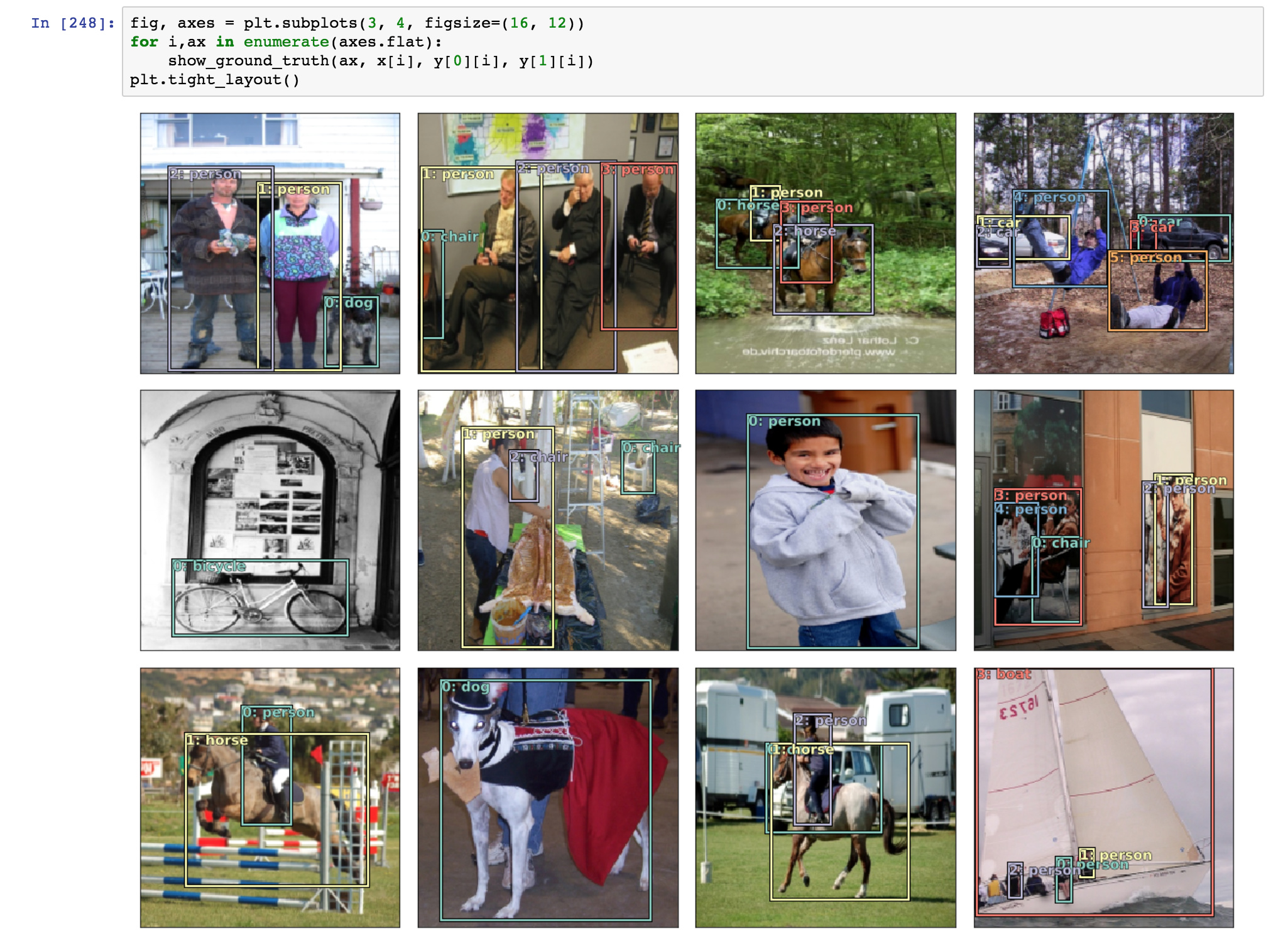
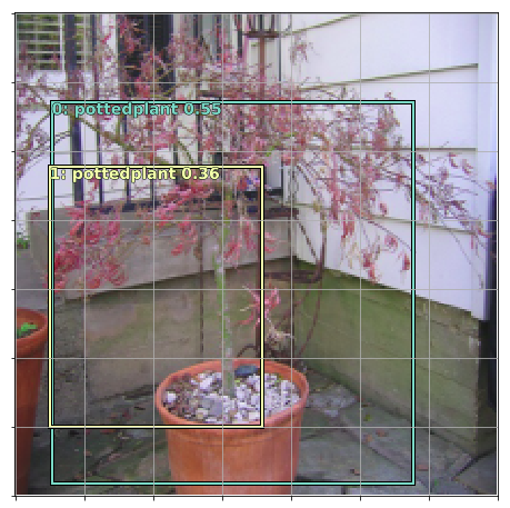
The below image depicts non max suppressed results. Initially, I thought it is incorrect - the smaller box is fully contained inside the bigger one so it should be suppressed. Then I realized - NMS will only suppress the less confident in its results prediction if its overlap with the other one ise > threshold. Meaning - if there will be an adequately small box inside a big box, the small box will not get suppressed. This is by design - if boxes are that much apart in sizes, the idea is that they might be predicting different objects and we do not wan to get rid of either of them.
I also ran into another reason why md.val_ds and val_mcs might not to line up - if the CSV file does not have the filenames in a sorted order. ImageClassifierData.from_csv sorts them while creating the training and validation sets. If we don’t sort the trn_ids similarly, they won’t line up correctly in the ConcatLblDataset…
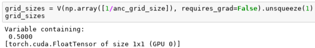
We use grid_sizes in the calculations to go from the activations to the predictions. So the gradient has to flow through them so that we can backpropagate the error. But this is essentially a constant. Why does it have to be a variable? Does it have to be a variable?
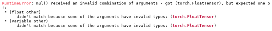
If I change grid_sizes to be a FloatTensor I get the error above. So seems it either wants a float or a Variable… mhmmm.
I realize that this will change in PyTorch 0.4, but could this be that gradients just cannot float through tensors that are not Variables?
I now tried running the code with grid_sizes being just a Python float and it works. So this seems like a limitation of PyTorch tensors that they can’t be used as constants? You either need a Variable or some numeric value as plain Tensors cannot be part of the computational graph as they lack some necessary functionality?
Edit: But we cannot keep the grid_sizes as a Python float since down the road we want different sizes of anchors per each grid cell… so if I am reading this right, because we cannot use floats in our situation, np.arrays cannot be part of the computational graph… Tensors are of limits cause they don’t allow the flow of gradients through them… we need to use Variables?
That’s basically right. The exact problem is that there are no ‘rank 0 tensors’ in pytorch. So scalars are considered ‘special’ - in the way you see above, amongst others. Really this should be a rank-0 variable, but that doesn’t exist.
Pytorch 0.4, I believe, will introduce rank 0 tensors. (And will get rid of variables, perhaps.)
In the detn_loss function why would it help to use a sigmoid activation to sqeeze the values between 0 and one and than multiply by 224?
Wouldn’t that make it much harder for the nn to get closer to the coordinates that are closer to the edge of the image?
I read in a paper that for binary classification, it is better to compare the result of the sigmoid to 0.2 for one class and 0.8 for the other instead of the 0 and 1 that is usually used. It is easier to approximate and causes less weight explosions. I think the same logic applies here. I can hopefully find the paper… please link it if anyone can, its from arxiv.
Yes sometimes I’ve tried something similar - e.g making the range -10 to 234, instead of 0 to 224, but I haven’t seen a clear improvement when doing so as yet.
it will make those zero-pads become boxes [0, 0, 1, 1], which in turn fails the condition check b[2]>0 and plots out those falsely aeroplane labels. So a simple way to fix is redefining bb_hw as
I have not idea why don’t rollback the parameters when the model have completely overfiting. At the first training, epoch 2 is trend to overfiting, and then keep training by lrs, the model have completely overfiting. In this case, I don’t know why we don’t rollback to result of the first training, because the second is overfitting!
In [12]:
lr = 2e-2
In [91]:
learn.fit(lr, 1, cycle_len=3, use_clr=(32,5))
A Jupyter Widget
epoch trn_loss val_loss
0 0.104836 0.085015 0.972356
1 0.088193 0.079739 0.972461
2 0.072346 0.077259 0.974114
Out[91]:
[0.077258907, 0.9741135761141777]
In [92]:
lrs = np.array([lr/100, lr/10, lr])
In [93]:
learn.freeze_to(-2)
In [135]:
learn.lr_find(lrs/1000)
learn.sched.plot(0)
Failed to display Jupyter Widget of type HBox.
If you’re reading this message in the Jupyter Notebook or JupyterLab Notebook, it may mean that the widgets JavaScript is still loading. If this message persists, it likely means that the widgets JavaScript library is either not installed or not enabled. See the Jupyter Widgets Documentation for setup instructions.
If you’re reading this message in another frontend (for example, a static rendering on GitHub or NBViewer), it may mean that your frontend doesn’t currently support widgets.
81%|█████████████████████████████████████████████████████████▋ | 26/32 [00:22<00:05, 1.15it/s, loss=0.33]
I’m trying to understand the implementation of focal loss, partly so I can port it to other areas. I’ve seen a few implementations online, but they all implement from scratch and the lesson 9 notebook it strikes me as particularly efficient given that it uses the weight parameter of the binary cross entropy function. I’d like to do the same for CE.
I want to confirm my understanding though that for focal loss we’re multiplying the cross entropy loss (-log(pt)) with a*(1-pt)^gamma and we can do that by setting weight in the F.cross_entropy_loss to that precalculated value.
def get_weight(self,x,t):
alpha,gamma = 0.25,1
p = x.sigmoid()
pt = p * t + (1-p) * (1-t)
w = alpha * t + (1-alpha) * (1-t)
return w * (1-pt).pow(gamma)
Similarly, I want to confirm we’re using sigmoid here because we’re doing BCE? And if I wanted to apply this to CE then the appropriate function would be .softmax() but the function would otherwise be identical?
I am using ‘Kaggle’ to run this code. But I am unable to use ‘ImageClassifierData.from_csv’ because I m unable to create a new ‘.csv’ file to save the dataframe ‘df’. Can anyone please help me in this scenario.