Hi All,
If you want the Jupyter notebook versions of the lecture notes, I have saved a versions on my github here.
Here’s lecture 4 notes. @vikbehal, I couldn’t edit your post, so I had to post another one. @jeremy, please turn this to a wiki thread so others can edit? Thank you!
Tim
Unofficial Deep Learning Lecture 4 Notes
Today’s topics - how to use the tools for these applications.
- Structured Learning
- Deep Learning for Language
- Deep Learning for Recommendation
Aside
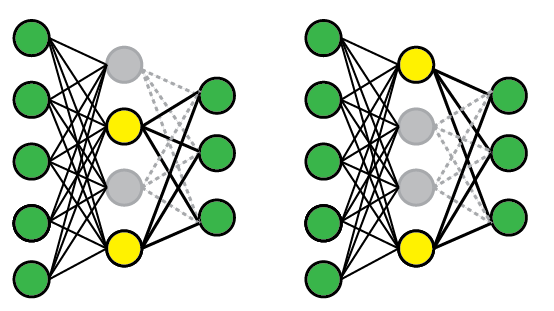
Dropout
Vocab
activations - A number that’s been calculated.
In lesson 2, Jeremy said, “An activation is a number saying the confidence of some level of, say, eyeballness.”. Activations are also sometimes referred to as parameters or features.
Looking at the Dog Breeds CNN model, let’s look at the different layers
Looking at Dogbreeds lets’ look at the layers:
(0)-BatchNorm
(1)-Dropout (p = 0.25) <----
(2)-Linear
(3)-ReLU
(4)-BatchNorm
(5)-Dropout (p = 0.5)
(6)-Linear
(7)-LogSoftMax
That means we go through and pick some activations and delete some of the calculated numbers.
p = whats the probability that you drop some cells.
Note: Each mini-batch we throw again a different set of activations.
- p = 0.00 - No drop
- p = 0.01 - will drop 1% of your activations (train well, but not very general)
- p = 0.99 - will drop out 99% of your activations, will kill your accuracy (super general)
If you find it overfitting, increase p.
As you start using bigger models you will probably need to increase the amount of dropout.
You may notice we have two linear layers. We’ve been adding 2 linear layers, xtra_fc=[] can handle this additional layer.
If we pass in the blank xfra_fc, we get a minimum model, which is the simplest sequential model:
(0)-BatchNorm
(1)-Linear
(2)-LogSoftMax
ps = [0, 0.2] can set the different drop out layers for the ConvLearner parameters
1. Structured and Time Series Data
%matplotlib inline
%reload_ext autoreload
%autoreload 2
import sys
sys.path.append('/home/paperspace/repos/fastai/')
import torch
from fastai.structured import *
from fastai.column_data import *
np.set_printoptions(threshold=50, edgeitems=20)

PATH='/home/paperspace/Desktop/data/rossman/'
Create datasets
We will look at the rossman kaggle competition as an example of structured data
In addition to the provided data, we will be using external datasets put together by participants in the Kaggle competition. You can download all of them here.
For completeness, the implementation used to put them together is included below.
def concat_csvs(dirname):
    path = f'{PATH}{dirname}'
    filenames=glob.glob(f"{path}/*.csv")

    wrote_header = False
    with open(f"{path}.csv","w") as outputfile:
        for filename in filenames:
            name = filename.split(".")[0]
            with open(filename) as f:
                line = f.readline()
                if not wrote_header:
                    wrote_header = True
                    outputfile.write("file,"+line)
                for line in f:
                     outputfile.write(name + "," + line)
                outputfile.write("\n")
Feature Space:
- train: Training set provided by competition
- store: List of stores
- store_states: mapping of store to the German state they are in
- List of German state names
- googletrend: trend of certain google keywords over time, found by users to correlate well w/ given data
- weather: weather
- test: testing set
table_names = ['train', 'store', 'store_states', 'state_names',
               'googletrend', 'weather', 'test']
We’ll be using the popular data manipulation framework pandas. Among other things, pandas allows you to manipulate tables/data frames in python as one would in a database.
We’re going to go ahead and load all of our csv’s as dataframes into the list tables.
tables = [pd.read_csv(f'{PATH}{fname}.csv', low_memory=False) for fname in table_names]
from IPython.display import HTML
We can use head() to get a quick look at the contents of each table:
- train: Contains store information on a daily basis, tracks things like sales, customers, whether that day was a holdiay, etc.
- store: general info about the store including competition, etc.
- store_states: maps store to state it is in
- state_names: Maps state abbreviations to names
- googletrend: trend data for particular week/state
- weather: weather conditions for each state
- test: Same as training table, w/o sales and customers
for t in tables: display(t.head())
| Store | DayOfWeek | Date | Sales | Customers | Open | Promo | StateHoliday | SchoolHoliday | |
|---|---|---|---|---|---|---|---|---|---|
| 0 | 1 | 5 | 2015-07-31 | 5263 | 555 | 1 | 1 | 0 | 1 |
| 1 | 2 | 5 | 2015-07-31 | 6064 | 625 | 1 | 1 | 0 | 1 |
| 2 | 3 | 5 | 2015-07-31 | 8314 | 821 | 1 | 1 | 0 | 1 |
| 3 | 4 | 5 | 2015-07-31 | 13995 | 1498 | 1 | 1 | 0 | 1 |
| 4 | 5 | 5 | 2015-07-31 | 4822 | 559 | 1 | 1 | 0 | 1 |
| Store | StoreType | Assortment | CompetitionDistance | CompetitionOpenSinceMonth | CompetitionOpenSinceYear | Promo2 | Promo2SinceWeek | Promo2SinceYear | PromoInterval | |
|---|---|---|---|---|---|---|---|---|---|---|
| 0 | 1 | c | a | 1270.0 | 9.0 | 2008.0 | 0 | NaN | NaN | NaN |
| 1 | 2 | a | a | 570.0 | 11.0 | 2007.0 | 1 | 13.0 | 2010.0 | Jan,Apr,Jul,Oct |
| 2 | 3 | a | a | 14130.0 | 12.0 | 2006.0 | 1 | 14.0 | 2011.0 | Jan,Apr,Jul,Oct |
| 3 | 4 | c | c | 620.0 | 9.0 | 2009.0 | 0 | NaN | NaN | NaN |
| 4 | 5 | a | a | 29910.0 | 4.0 | 2015.0 | 0 | NaN | NaN | NaN |
| Store | State | |
|---|---|---|
| 0 | 1 | HE |
| 1 | 2 | TH |
| 2 | 3 | NW |
| 3 | 4 | BE |
| 4 | 5 | SN |
| StateName | State | |
|---|---|---|
| 0 | BadenWuerttemberg | BW |
| 1 | Bayern | BY |
| 2 | Berlin | BE |
| 3 | Brandenburg | BB |
| 4 | Bremen | HB |
| file | week | trend | |
|---|---|---|---|
| 0 | Rossmann_DE_SN | 2012-12-02 - 2012-12-08 | 96 |
| 1 | Rossmann_DE_SN | 2012-12-09 - 2012-12-15 | 95 |
| 2 | Rossmann_DE_SN | 2012-12-16 - 2012-12-22 | 91 |
| 3 | Rossmann_DE_SN | 2012-12-23 - 2012-12-29 | 48 |
| 4 | Rossmann_DE_SN | 2012-12-30 - 2013-01-05 | 67 |
| file | Date | Max_TemperatureC | Mean_TemperatureC | Min_TemperatureC | Dew_PointC | MeanDew_PointC | Min_DewpointC | Max_Humidity | Mean_Humidity | ... | Max_VisibilityKm | Mean_VisibilityKm | Min_VisibilitykM | Max_Wind_SpeedKm_h | Mean_Wind_SpeedKm_h | Max_Gust_SpeedKm_h | Precipitationmm | CloudCover | Events | WindDirDegrees | |
|---|---|---|---|---|---|---|---|---|---|---|---|---|---|---|---|---|---|---|---|---|---|
| 0 | NordrheinWestfalen | 2013-01-01 | 8 | 4 | 2 | 7 | 5 | 1 | 94 | 87 | ... | 31.0 | 12.0 | 4.0 | 39 | 26 | 58.0 | 5.08 | 6.0 | Rain | 215 |
| 1 | NordrheinWestfalen | 2013-01-02 | 7 | 4 | 1 | 5 | 3 | 2 | 93 | 85 | ... | 31.0 | 14.0 | 10.0 | 24 | 16 | NaN | 0.00 | 6.0 | Rain | 225 |
| 2 | NordrheinWestfalen | 2013-01-03 | 11 | 8 | 6 | 10 | 8 | 4 | 100 | 93 | ... | 31.0 | 8.0 | 2.0 | 26 | 21 | NaN | 1.02 | 7.0 | Rain | 240 |
| 3 | NordrheinWestfalen | 2013-01-04 | 9 | 9 | 8 | 9 | 9 | 8 | 100 | 94 | ... | 11.0 | 5.0 | 2.0 | 23 | 14 | NaN | 0.25 | 7.0 | Rain | 263 |
| 4 | NordrheinWestfalen | 2013-01-05 | 8 | 8 | 7 | 8 | 7 | 6 | 100 | 94 | ... | 10.0 | 6.0 | 3.0 | 16 | 10 | NaN | 0.00 | 7.0 | Rain | 268 |
5 rows × 24 columns
| Id | Store | DayOfWeek | Date | Open | Promo | StateHoliday | SchoolHoliday | |
|---|---|---|---|---|---|---|---|---|
| 0 | 1 | 1 | 4 | 2015-09-17 | 1.0 | 1 | 0 | 0 |
| 1 | 2 | 3 | 4 | 2015-09-17 | 1.0 | 1 | 0 | 0 |
| 2 | 3 | 7 | 4 | 2015-09-17 | 1.0 | 1 | 0 | 0 |
| 3 | 4 | 8 | 4 | 2015-09-17 | 1.0 | 1 | 0 | 0 |
| 4 | 5 | 9 | 4 | 2015-09-17 | 1.0 | 1 | 0 | 0 |
Data Cleaning / Feature Engineering
As a structured data problem, we necessarily have to go through all the cleaning and feature engineering, even though we’re using a neural network.
These are the consolidated Data processing blocks. For the originals, please refer to lesson 4 on deep learning.
train, store, store_states, state_names, googletrend, weather, test = tables
len(train),len(test)
We turn state Holidays to booleans, to make them more convenient for modeling. We can do calculations on pandas fields using notation very similar (often identical) to numpy.
Data Processing Blocks
train.StateHoliday = train.StateHoliday!='0'
test.StateHoliday = test.StateHoliday!='0'

def join_df(left, right, left_on, right_on=None, suffix='_y'):
    if right_on is None: right_on = left_on
    return left.merge(right, how='left', left_on=left_on, right_on=right_on,
                      suffixes=("", suffix))

weather = join_df(weather, state_names, "file", "StateName")

googletrend['Date'] = googletrend.week.str.split(' - ', expand=True)[0]
googletrend['State'] = googletrend.file.str.split('_', expand=True)[2]
googletrend.loc[googletrend.State=='NI', "State"] = 'HB,NI'

add_datepart(weather, "Date", drop=False)
add_datepart(googletrend, "Date", drop=False)
add_datepart(train, "Date", drop=False)
add_datepart(test, "Date", drop=False)
add_datepart(googletrend, "Date", drop=False)

trend_de = googletrend[googletrend.file == 'Rossmann_DE']

store = join_df(store, store_states, "Store")
len(store[store.State.isnull()])

joined = join_df(train, store, "Store")
len(joined[joined.StoreType.isnull()])

joined = join_df(joined, googletrend, ["State","Year", "Week"])
len(joined[joined.trend.isnull()])

joined = joined.merge(trend_de, 'left', ["Year", "Week"], suffixes=('', '_DE'))
len(joined[joined.trend_DE.isnull()])

joined = join_df(joined, weather, ["State","Date"])
len(joined[joined.Mean_TemperatureC.isnull()])

joined_test = test.merge(store, how='left', left_on='Store', right_index=True)
len(joined_test[joined_test.StoreType.isnull()])

for c in joined.columns:
    if c.endswith('_y'):
        if c in joined.columns: joined.drop(c, inplace=True, axis=1)
joined.CompetitionOpenSinceYear = joined.CompetitionOpenSinceYear.fillna(1900).astype(np.int32)
joined.CompetitionOpenSinceMonth = joined.CompetitionOpenSinceMonth.fillna(1).astype(np.int32)
joined.Promo2SinceYear = joined.Promo2SinceYear.fillna(1900).astype(np.int32)
joined.Promo2SinceWeek = joined.Promo2SinceWeek.fillna(1).astype(np.int32)

joined["CompetitionOpenSince"] = pd.to_datetime(dict(year=joined.CompetitionOpenSinceYear,
                                                     month=joined.CompetitionOpenSinceMonth, day=15))
joined["CompetitionDaysOpen"] = joined.Date.subtract(joined.CompetitionOpenSince).dt.days

joined.loc[joined.CompetitionDaysOpen<0, "CompetitionDaysOpen"] = 0
joined.loc[joined.CompetitionOpenSinceYear<1990, "CompetitionDaysOpen"] = 0

joined["CompetitionMonthsOpen"] = joined["CompetitionDaysOpen"]//30
joined.loc[joined.CompetitionMonthsOpen>24, "CompetitionMonthsOpen"] = 24
joined.CompetitionMonthsOpen.unique()

joined["Promo2Since"] = pd.to_datetime(joined.apply(lambda x: Week(
    x.Promo2SinceYear, x.Promo2SinceWeek).monday(), axis=1).astype(pd.datetime))
joined["Promo2Days"] = joined.Date.subtract(joined["Promo2Since"]).dt.days

joined.loc[joined.Promo2Days<0, "Promo2Days"] = 0
joined.loc[joined.Promo2SinceYear<1990, "Promo2Days"] = 0


joined["Promo2Weeks"] = joined["Promo2Days"]//7
joined.loc[joined.Promo2Weeks<0, "Promo2Weeks"] = 0
joined.loc[joined.Promo2Weeks>25, "Promo2Weeks"] = 25
joined.Promo2Weeks.unique()

joined.to_feather(f'{PATH}joined')
def get_elapsed(fld, pre):
    day1 = np.timedelta64(1, 'D')
    last_date = np.datetime64()
    last_store = 0
    res = []

    for s,v,d in zip(df.Store.values,df[fld].values, df.Date.values):
        if s != last_store:
            last_date = np.datetime64()
            last_store = s
        if v: last_date = d
        res.append(((d-last_date).astype('timedelta64[D]') / day1).astype(int))
    df[pre+fld] = res


columns = ["Date", "Store", "Promo", "StateHoliday", "SchoolHoliday"]
df = train[columns]

fld = 'SchoolHoliday'
df = df.sort_values(['Store', 'Date'])
get_elapsed(fld, 'After')
df = df.sort_values(['Store', 'Date'], ascending=[True, False])
get_elapsed(fld, 'Before')

fld = 'StateHoliday'
df = df.sort_values(['Store', 'Date'])
get_elapsed(fld, 'After')
df = df.sort_values(['Store', 'Date'], ascending=[True, False])
get_elapsed(fld, 'Before')

fld = 'Promo'
df = df.sort_values(['Store', 'Date'])
get_elapsed(fld, 'After')
df = df.sort_values(['Store', 'Date'], ascending=[True, False])
get_elapsed(fld, 'Before')

df = df.set_index("Date")

columns = ['SchoolHoliday', 'StateHoliday', 'Promo']

for o in ['Before', 'After']:
    for p in columns:
        a = o+p
        df[a] = df[a].fillna(0)

bwd = df[['Store']+columns].sort_index().groupby("Store").rolling(7, min_periods=1).sum()
fwd = df[['Store']+columns].sort_index(ascending=False
                                      ).groupby("Store").rolling(7, min_periods=1).sum()

bwd.drop('Store',1,inplace=True)
bwd.reset_index(inplace=True)

fwd.drop('Store',1,inplace=True)
fwd.reset_index(inplace=True)

df.reset_index(inplace=True)

df = df.merge(bwd, 'left', ['Date', 'Store'], suffixes=['', '_bw'])
df = df.merge(fwd, 'left', ['Date', 'Store'], suffixes=['', '_fw'])

df.drop(columns,1,inplace=True)
df.to_csv(f'{PATH}df.csv')
df.head()
df["Date"] = pd.to_datetime(df.Date)
df.columns
Index(['Date', 'Store', 'AfterSchoolHoliday', 'BeforeSchoolHoliday',
       'AfterStateHoliday', 'BeforeStateHoliday', 'AfterPromo', 'BeforePromo',
       'SchoolHoliday_bw', 'StateHoliday_bw', 'Promo_bw', 'SchoolHoliday_fw',
       'StateHoliday_fw', 'Promo_fw'],
      dtype='object')
joined = join_df(joined, df, ['Store', 'Date'])
joined = joined[joined.Sales!=0]
joined.reset_index(inplace=True)
joined.to_feather(f'{PATH}joined')
Check point! Save your feather file!
joined = pd.read_feather(f'{PATH}joined')
Discussion on Categorical
Which say which are categorical / continuous. This is a decision that we are going to make. Sometimes there are variables that are directly coded as categorical, there’s only one choice. But continuous in the data, you can make a decision.
For the 3rd place team, most of the continuous ones are mainly the floating point numbers. The number of levels in a category is the cardinality. We could bin variables 10 → 100 into 10-20, 20-30, etc.
cat_vars = ['Store', 'DayOfWeek', 'Year', 'Month', 'Day', 'StateHoliday', 'CompetitionMonthsOpen',
    'Promo2Weeks', 'StoreType', 'Assortment', 'PromoInterval', 'CompetitionOpenSinceYear', 'Promo2SinceYear',
    'State', 'Week', 'Events', 'Promo_fw', 'Promo_bw', 'StateHoliday_fw', 'StateHoliday_bw',
    'SchoolHoliday_fw', 'SchoolHoliday_bw']

contin_vars = ['CompetitionDistance', 'Max_TemperatureC', 'Mean_TemperatureC', 'Min_TemperatureC',
   'Max_Humidity', 'Mean_Humidity', 'Min_Humidity', 'Max_Wind_SpeedKm_h',
   'Mean_Wind_SpeedKm_h', 'CloudCover', 'trend', 'trend_DE',
   'AfterStateHoliday', 'BeforeStateHoliday', 'Promo', 'SchoolHoliday']

n = len(joined); n
844338
Now we can loop through and change them all into categorical
Turn all the continuous ones into 32bit floating point for pytorch’s sake
for v in cat_vars: joined[v] = joined[v].astype('category').cat.as_ordered()
for v in contin_vars: joined[v] = joined[v].astype('float32')
dep = 'Sales'
joined = joined[cat_vars+contin_vars+[dep, 'Date']]
idxs = get_cv_idxs(n, val_pct=150000/n)
joined_samp = joined.iloc[idxs].set_index("Date")
samp_size = len(joined_samp); samp_size
150000
Get a smaller sample size
samp_size = n
joined_samp = joined.set_index("Date")
joined_samp.head(2)
| Store | DayOfWeek | Year | Month | Day | StateHoliday | CompetitionMonthsOpen | Promo2Weeks | StoreType | Assortment | ... | Max_Wind_SpeedKm_h | Mean_Wind_SpeedKm_h | CloudCover | trend | trend_DE | AfterStateHoliday | BeforeStateHoliday | Promo | SchoolHoliday | Sales | |
|---|---|---|---|---|---|---|---|---|---|---|---|---|---|---|---|---|---|---|---|---|---|
| Date | |||||||||||||||||||||
| 2015-07-31 | 1 | 5 | 2015 | 7 | 31 | False | 24 | 0 | c | a | ... | 24.0 | 11.0 | 1.0 | 85.0 | 83.0 | 57.0 | -9.223372e+18 | 1.0 | 1.0 | 5263 |
| 2015-07-31 | 2 | 5 | 2015 | 7 | 31 | False | 24 | 25 | a | a | ... | 14.0 | 11.0 | 4.0 | 80.0 | 83.0 | 67.0 | -9.223372e+18 | 1.0 | 1.0 | 6064 |
2 rows × 39 columns
Fastai Process Dataframe
proc_df- pulls out the target (y) and deletes from the original.- Also scales the dataframe.
- Also creates another object to keep track of std and mean for changing the test set.
- Also handles missing values, fills with median.
df, y, nas, mapper = proc_df(joined_samp, 'Sales', do_scale=True)
yl = np.log(y)
train_ratio = 0.75
# train_ratio = 0.9
train_size = int(samp_size * train_ratio); train_size
val_idx = list(range(train_size, len(df)))
val_idx = np.flatnonzero(
    (df.index<=datetime.datetime(2014,9,17)) & (df.index>=datetime.datetime(2014,8,1)))
Validation Set - Last two weeks
Make it as similar dataset as possible. This won’t be a random set like other times because this is time series.
The Deep Learning Version
def inv_y(a): return np.exp(a)

def exp_rmspe(y_pred, targ):
    targ = inv_y(targ)
    pct_var = (targ - inv_y(y_pred))/targ
    return math.sqrt((pct_var**2).mean())

max_log_y = np.max(yl)
y_range = (0, max_log_y*1.2)
Very similar to the image recognition process
- find training dataset
- find test set
- set a learner
- fit and go
But since we are not doing images, but structured data: ColumnarModelData
PATH- where to store everything that you save laterval_idx- which we will put in the validation setdf- dataframeyl- target (dependent variable)cat_flds- which things we want to treat as categorical. At this time everything is a number
md = ColumnarModelData.from_data_frame(PATH, val_idx, df, yl, cat_flds=cat_vars, bs=128)
Jumping ahead we need to set the learner …
- How much drop out
- How many embeddings
m = md.get_learner(emb_szs, len(df.columns)-len(cat_vars),
                   0.04, 1, [1000,500], [0.001,0.01], y_range=y_range)
lr = 1e-3
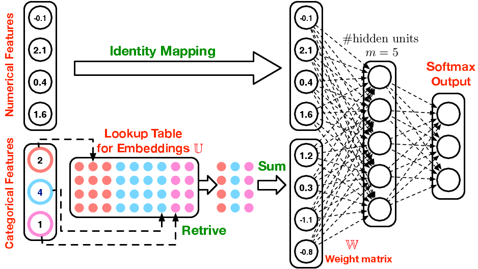
New Topic: Embeddings
The continuous variables, we are going to grab them all.
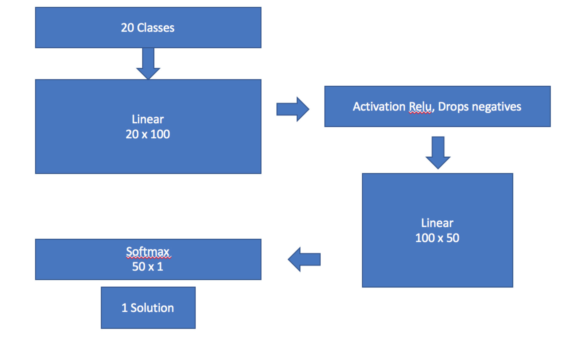
What if you had days of the week, lets assign 4 random numbers.
- 0-Sunday
- 1-Mon
- 2-Tue
- 3-Wed
- 4-Thu
- 5-Fri
- 6-Sat
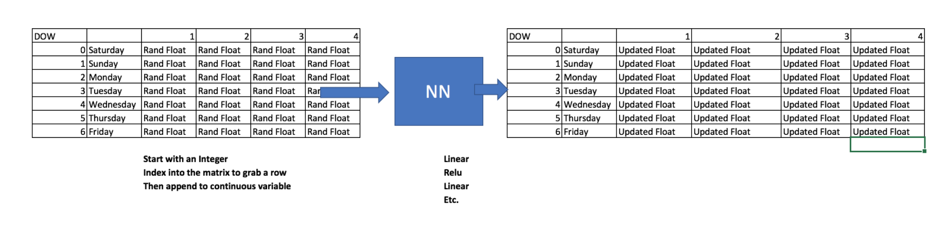
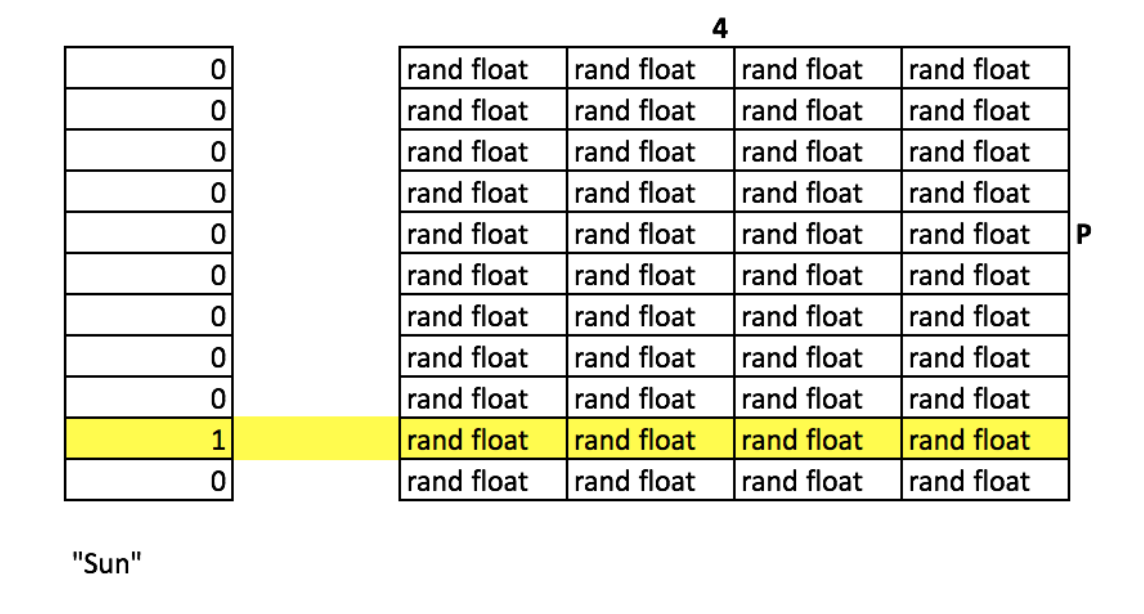
Where did 4 come from for Day of Week?
What’s our Cardinality for our Categorical Variables?
cat_sz = [(c, len(joined_samp[c].cat.categories)+1) for c in cat_vars]
cat_sz
[('Store', 1116),
 ('DayOfWeek', 8),
 ('Year', 4),
 ('Month', 13),
 ('Day', 32),
 ('StateHoliday', 3),
 ('CompetitionMonthsOpen', 26),
 ('Promo2Weeks', 27),
 ('StoreType', 5),
 ('Assortment', 4),
 ('PromoInterval', 4),
 ('CompetitionOpenSinceYear', 24),
 ('Promo2SinceYear', 9),
 ('State', 13),
 ('Week', 53),
 ('Events', 22),
 ('Promo_fw', 7),
 ('Promo_bw', 7),
 ('StateHoliday_fw', 4),
 ('StateHoliday_bw', 4),
 ('SchoolHoliday_fw', 9),
 ('SchoolHoliday_bw', 9)]
Rough Formula : Take your cardinality, divide by 2, but not more than 50
emb_szs = [(c, min(50, (c+1)//2)) for _,c in cat_sz]
emb_szs
[(1116, 50),
 (8, 4),
 (4, 2),
 (13, 7),
 (32, 16),
 (3, 2),
 (26, 13),
 (27, 14),
 (5, 3),
 (4, 2),
 (4, 2),
 (24, 12),
 (9, 5),
 (13, 7),
 (53, 27),
 (22, 11),
 (7, 4),
 (7, 4),
 (4, 2),
 (4, 2),
 (9, 5),
 (9, 5)]
Embedding = Distributed Representation
Jumping ahead we need to set the learner …
emb_szsOur embeddingslen(df.columns)-len(cat_vars)- how many continous variables[1000,500]activations in linear layer[0.001,0.01]- drop outs per linear layer1- our output
m = md.get_learner(emb_szs, len(df.columns)-len(cat_vars),
                   0.04, 1, [1000,500], [0.001,0.01], y_range=y_range)
lr = 1e-3
m = md.get_learner(emb_szs, len(df.columns)-len(cat_vars),
                   0.04, 1, [1000,500], [0.001,0.01], y_range=y_range)
lr = 1e-3
m.fit(lr, 3, metrics=[exp_rmspe])
[ 0.       0.02479  0.02205  0.19309]
[ 1.       0.02044  0.01751  0.18301]
[ 2.       0.01598  0.01571  0.17248]
m.fit(lr, 1, metrics=[exp_rmspe], cycle_len=1)
[ 0. 0.00676 0.01041 0.09711]
Step Overall
- List the Categorical
- List of row indexes in your dataset
- Call the
columnar dataset - How big you want your embedding matrix
- Get learner
- Fit
2. Deep Learning for Language
Language Modeling
Can you predict what the next word is going to be? Swiftkey actually does this. Modeling predicts the next word.
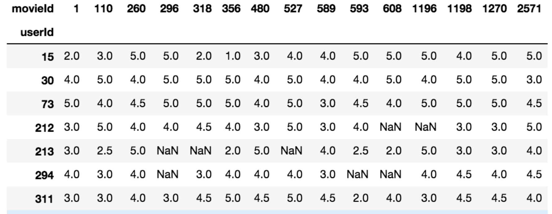
IMDb movie review dataset
http://ai.stanford.edu/~amaas/data/sentiment/
#!pip install spacy
To download the ‘en’ library needed, run:
#!python -m spacy download en
The large movie view dataset contains a collection of 50,000 reviews from IMDB. The dataset contains an even number of positive and negative reviews. The authors considered only highly polarized reviews. A negative review has a score ≤ 4 out of 10, and a positive review has a score ≥ 7 out of 10. Neutral reviews are not included in the dataset. The dataset is divided into training and test sets. The training set is the same 25,000 labeled reviews.
The sentiment classification task consists of predicting the polarity (positive or negative) of a given text.
However, before we try to classify sentiment, we will simply try to create a language model; that is, a model that can predict the next word in a sentence. Why? Because our model first needs to understand the structure of English, before we can expect it to recognize positive vs negative sentiment.
So our plan of attack is the same as we used for Dogs v Cats: pretrain a model to do one thing (predict the next word), and fine tune it to do something else (classify sentiment).
Unfortunately, there are no good pretrained language models available to download, so we need to create our own.
import torch
%reload_ext autoreload
%autoreload 2
%matplotlib inline

import sys
sys.path.append('/home/paperspace/repos/fastai/')

from fastai.imports import *
from fastai.torch_imports import *
from fastai.core import *
from fastai.model import fit
from fastai.dataset import *

import torchtext
from torchtext import vocab, data
from torchtext.datasets import language_modeling

from fastai.rnn_reg import *
from fastai.rnn_train import *
from fastai.nlp import *
from fastai.lm_rnn import *

import dill as pickle
Torchtext - is Pytorch’s NLP library
PATH='/home/paperspace/Desktop/data/imdb/aclImdb/'

TRN_PATH = 'train/all/'
VAL_PATH = 'test/all/'
TRN = f'{PATH}{TRN_PATH}'
VAL = f'{PATH}{VAL_PATH}'

%ls {PATH}
imdbEr.txt imdb.vocab emodelse/ README etest/ etmp/ etrain/
trn_files = !ls {TRN}
trn_files[:10]
['0_0.txt',
 '0_3.txt',
 '0_9.txt',
 '10000_0.txt',
 '10000_4.txt',
 '10000_8.txt',
 '1000_0.txt',
 '10001_0.txt',
 '10001_10.txt',
 '10001_4.txt']
review = !cat {TRN}{trn_files[6]}
review[0]
"I have to say when a name like Zombiegeddon and an atom bomb on the front cover I was expecting a flat out chop-socky fung-ku, but what I got instead was a comedy. So, it wasn't quite was I was expecting, but I really liked it anyway! The best scene ever was the main cop dude pulling those kids over and pulling a Bad Lieutenant on them!! I was laughing my ass off. I mean, the cops were just so bad! And when I say bad, I mean The Shield Vic Macky bad. But unlike that show I was laughing when they shot people and smoked dope.<br /><br />Felissa Rose...man, oh man. What can you say about that hottie. She was great and put those other actresses to shame. She should work more often!!!!! I also really liked the fight scene outside of the building. That was done really well. Lots of fighting and people getting their heads banged up. FUN! Last, but not least Joe Estevez and William Smith were great as the...well, I wasn't sure what they were, but they seemed to be having fun and throwing out lines. I mean, some of it didn't make sense with the rest of the flick, but who cares when you're laughing so hard! All in all the film wasn't the greatest thing since sliced bread, but I wasn't expecting that. It was a Troma flick so I figured it would totally suck. It's nice when something surprises you but not totally sucking.<br /><br />Rent it if you want to get stoned on a Friday night and laugh with your buddies. Don't rent it if you are an uptight weenie or want a zombie movie with lots of flesh eating.<br /><br />P.S. Uwe Boil was a nice touch."
!find {TRN} -name '*.txt' | xargs cat | wc -w
17486581
!find {VAL} -name '*.txt' | xargs cat | wc -w
5686719
' '.join(spacy_tok(review[0]))
"I have to say when a name like Zombiegeddon and an atom bomb on the front cover I was expecting a flat out chop - socky fung - ku , but what I got instead was a comedy . So , it was n't quite was I was expecting , but I really liked it anyway ! The best scene ever was the main cop dude pulling those kids over and pulling a Bad Lieutenant on them ! ! I was laughing my ass off . I mean , the cops were just so bad ! And when I say bad , I mean The Shield Vic Macky bad . But unlike that show I was laughing when they shot people and smoked dope . \n\n Felissa Rose ... man , oh man . What can you say about that hottie . She was great and put those other actresses to shame . She should work more often ! ! ! ! ! I also really liked the fight scene outside of the building . That was done really well . Lots of fighting and people getting their heads banged up . FUN ! Last , but not least Joe Estevez and William Smith were great as the ... well , I was n't sure what they were , but they seemed to be having fun and throwing out lines . I mean , some of it did n't make sense with the rest of the flick , but who cares when you 're laughing so hard ! All in all the film was n't the greatest thing since sliced bread , but I was n't expecting that . It was a Troma flick so I figured it would totally suck . It 's nice when something surprises you but not totally sucking . \n\n Rent it if you want to get stoned on a Friday night and laugh with your buddies . Do n't rent it if you are an uptight weenie or want a zombie movie with lots of flesh eating . \n\n P.S. Uwe Boil was a nice touch ."
We use Pytorch’s torchtext library to pre-process our data, telling it to use the wonderful spacy library to handle tokenization.
First, we create a torchtext field, which describes how to pre-process a piece of text - in this case, we tell torchtext to make everything lowercase, and tokenize it with spacy.
we will lower, then we will spacy tokenize.
TEXT = data.Field(lower=True, tokenize=spacy_tok)
fastai library works closely with torchtext. We create a ModelData object for language modeling by taking advantage of LanguageModelData, passing it our torchtext field object, and the paths to our training, test, and validation sets. In this case, we don’t have a separate test set, so we’ll just use VAL_PATH for that too.
As well as the usual bs (batch size) parameter, we also not have bptt; this define how many words are processing at a time in each row of the mini-batch. More importantly, it defines how many ‘layers’ we will backprop through. Making this number higher will increase time and memory requirements, but will improve the model’s ability to handle long sentences.
min_freq- must occur with 10 timesbs- batch sizebptt- back propagation (through time) - how much of the sentence will sit at any time
bs=64; bptt=70

WARNING: takes a long time to run
FILES = dict(train=TRN_PATH, validation=VAL_PATH, test=VAL_PATH)
md = LanguageModelData(PATH, TEXT, **FILES, bs=bs, bptt=bptt, min_freq=10)
After building our ModelData object, it automatically fills the TEXT object with a very important attribute: TEXT.vocab. This is a vocabulary, which stores which words (or tokens) have been seen in the text, and how each word will be mapped to a unique integer id. We’ll need to use this information again later, so we save it.
(Technical note: python’s standard Pickle library can’t handle this correctly, so at the top of this notebook we used the dill library instead and imported it as pickle).
Save the model for later
pickle.dump(TEXT, open(f'{PATH}models/TEXT.pkl','wb'))
Here are the: # batches; # unique tokens in the vocab; # tokens in the training set; # sentences
len(md.trn_dl), md.nt, len(md.trn_ds), len(md.trn_ds[0].text)
(4603, 34933, 1, 20626672)
This is the start of the mapping from integer IDs to unique tokens.
# 'itos': 'int-to-string'
TEXT.vocab.itos[:12]
['<unk>', '<pad>', 'the', ',', '.', 'and', 'a', 'of', 'to', 'is', 'it', 'in']
# 'stoi': 'string to int'
TEXT.vocab.stoi['the']
2
Note that in a LanguageModelData object there is only one item in each dataset: all the words of the text joined together.
TEXT.numericalize([md.trn_ds[0].text[:12]])
Variable containing:
   37
  866
    3
   27
  194
   67
    3
    2
  378
    3
   27
  194
[torch.cuda.LongTensor of size 12x1 (GPU 0)]
Our LanguageModelData object will create batches with 64 columns (that’s our batch size), and varying sequence lengths of around 80 tokens (that’s our bptt parameter - backprop through time).
Each batch also contains the exact same data as labels, but one word later in the text - since we’re trying to always predict the next word. The labels are flattened into a 1d array.
next(iter(md.trn_dl))
(Variable containing:
     37    409     22  ...      50     56      4
    866    232      6  ...     815     51     34
      3    584    655  ...       4     59    325
         ...            ⋱           ...
     44     60   2332  ...      14    841   9681
   2768     10      9  ...      75      3    360
   1032    149    899  ...   12254      6     14
 [torch.cuda.LongTensor of size 81x64 (GPU 0)], Variable containing:
    866
    232
      6
   ⋮
     32
    865
     27
 [torch.cuda.LongTensor of size 5184 (GPU 0)])
Let’s make our own Embedding off of our data
md.nt= number of tokens = 34,495md.trn_ds[0].text= 20,621,966
Train
We have a number of parameters to set - we’ll learn more about these later, but you should find these values suitable for many problems.
em_sz = 200  # size of each embedding vector
nh = 500     # number of hidden activations per layer
nl = 3       # number of layers
Researchers have found that large amounts of momentum (which we’ll learn about later) don’t work well with these kinds of RNN models, so we create a version of the Adam optimizer with less momentum than it’s default of 0.9.
Adam Optimizer, the defaults don’t work very well
opt_fn = partial(optim.Adam, betas=(0.7, 0.99))
fastai library uses a variant of the state of the art AWD LSTM Language Model developed by Stephen Merity. A key feature of this model is that it provides excellent regularization through Dropout. There is no simple way known (yet!) to find the best values of the dropout parameters below - you just have to experiment…
However, the other parameters (alpha, beta, and clip) shouldn’t generally need tuning.
opt_fn- defaults for adam optimizerem_sz- embedding sizenh- number of activationsnl- number of layersdropout- how much drop out to add (won’t elaborate)learner.clip=0.3- don’t let the gradient go any lower than this number
This is a RNN using an LSTM
learner = md.get_model(opt_fn, em_sz, nh, nl,
               dropouti=0.05, dropout=0.05, wdrop=0.1, dropoute=0.02, dropouth=0.05)
learner.reg_fn = partial(seq2seq_reg, alpha=2, beta=1)
learner.clip=0.3
As you can see below, I gradually tuned the language model in a few stages. I possibly could have trained it further (it wasn’t yet overfitting), but I didn’t have time to experiment more. Maybe you can see if you can train it to a better accuracy! (I used lr_find to find a good learning rate, but didn’t save the output in this notebook. Feel free to try running it yourself now.)
Trying different settings and modeling
learner.fit(3e-3, 1, wds=1e-6, cycle_len=20, cycle_save_name='adam3_20')
[ 0.       6.44582  6.40362]
[ 1.       4.71655  4.61361]
[ 2.       4.59772  4.49624]
[ 3.       4.53644  4.44157]
[ 4.       4.5055   4.40163]
[ 5.       4.47234  4.37386]
[ 6.       4.44514  4.35307]
[ 7.       4.42154  4.33165]
[ 8.       4.39408  4.31588]
[ 9.       4.38333  4.30152]
[ 10.        4.35194   4.28591]
[ 11.        4.35191   4.27355]
[ 12.        4.32064   4.25818]
[ 13.        4.29965   4.2474 ]
[ 14.        4.28177   4.23785]
[ 15.        4.28475   4.23243]
[ 16.        4.25953   4.22698]
[ 17.        4.23739   4.22239]
[ 18.        4.24809   4.22182]
[ 19.        4.25874   4.22156]
learner.load_cycle('adam3_20', 0)
learner.save_encoder('adam3_20_enc')
Sentiment
We’ll need to the saved vocab from the language model, since we need to ensure the same words map to the same IDs.
TEXT = pickle.load(open(f'{PATH}models/TEXT.pkl','rb'))
sequential=False tells torchtext that a text field should be tokenized (in this case, we just want to store the ‘positive’ or ‘negative’ single label).
splits is a torchtext method that creates train, test, and validation sets. The IMDB dataset is built into torchtext, so we can take advantage of that. Take a look at lang_model-arxiv.ipynb to see how to define your own fastai/torchtext datasets.
IMDB_LABEL = data.Field(sequential=False)
splits = torchtext.datasets.IMDB.splits(TEXT, IMDB_LABEL, 'data/')
t = splits[0].examples[0]
t.label, ' '.join(t.text[:16])
('pos',
 'i remember watching this movie with my friends when we were 4 years old , but')
fastai library can create a ModelData object directly from torchtext splits.
md2 = TextData.from_splits(PATH, splits, bs)
m3 = md2.get_model(opt_fn, 1500, bptt, emb_sz=em_sz, n_hid=nh, n_layers=nl,
           dropout=0.1, dropouti=0.4, wdrop=0.5, dropoute=0.05, dropouth=0.3)
m3.reg_fn = partial(seq2seq_reg, alpha=2, beta=1)
m3.load_encoder(f'adam3_20_enc')
Because we’re fine-tuning a pretrained model, we’ll use differential learning rates, and also increase the max gradient for clipping, to allow the SGDR to work better.
m3.clip=25.
lrs=np.array([1e-4,1e-3,1e-2])
3. Deep Learning for Recommendation
Next week, we will be learning Collaborative Filtering and making this.