Unofficial Lecture 10 Notes
Hi all, hope these notes are useful. This is from the morning version of the lecture.
- Tim
Logistic Regression
%reload_ext autoreload
%autoreload 2
%matplotlib inline

from fastai.nlp import *
from sklearn.linear_model import LogisticRegression
# from torchtext import vocab, data, datasets
PATH='aclImdb/'
names = ['neg','pos']
trn,trn_y = texts_from_folders(f'{PATH}train',names)
val,val_y = texts_from_folders(f'{PATH}test',names)
veczr = CountVectorizer(tokenizer=tokenize)
trn_term_doc = veczr.fit_transform(trn)
val_term_doc = veczr.transform(val)
x=trn_term_doc
y=trn_y
Recapping the Logistic Regression (C = constant)
Make sure you have a lot of parameters. Linear models can work sometimes, if the underlying assumption of linearity isn’t too bad. Works much better with neural networks and more hidden layers.
For sentiment, if you look at a set of words, only need a few words to tell us if the documents is either happy or sad. Have lots of parameters and use regularization
m = LogisticRegression(C=1e8, dual=True)
m.fit(x, y)
preds = m.predict(val_term_doc)
(preds==val_y).mean()
0.85511999999999999
Trigrams

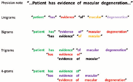
veczr =  CountVectorizer(ngram_range=(1,3), tokenizer=tokenize, max_features=800000)
trn_term_doc = veczr.fit_transform(trn)
val_term_doc = veczr.transform(val)
x=trn_term_doc
y=trn_y
Note: the x input is all 0, or counts
x = [[3 0 0 1...
      0 0 0 1
      0 2 1 0   ]]
m = LogisticRegression(C=1e8, dual=True)
m.fit(x, y)
preds = m.predict(val_term_doc)
(preds==val_y).mean()
0.89903999999999995
From Naive Bays
y=trn_y
x=trn_term_doc.sign()
val_x = val_term_doc.sign()

p = x[y==1].sum(0)+1
q = x[y==0].sum(0)+1
r = np.log((p/p.sum())/(q/q.sum()))
b = np.log(len(p)/len(q))
vocab = veczr.get_feature_names()
How happy or sad everything is
np.exp(r)
matrix([[ 0.95208, 0.85605, 0.78485, ..., 3.01678, 0.5028 , 0.5028 ]])
vocab[-3]
'” .'
vocab[3]
'! ! "'
All the ones will be replaced with the log count ratio
Now consider a different input
x = [[0 0    0    0.45 ...
      0 0    0    0.45
      0 0.65 0.45 0   ]]
x_nb = x.multiply(r)
m = LogisticRegression(dual=True, C=0.1)
m.fit(x_nb, y);

val_x_nb = val_x.multiply(r)
preds = m.predict(val_x_nb)
(preds.T==val_y).mean()
0.91768000000000005
Why is the binarized version better
the r measure is a good estimate of how positive or negative it is. Regularization moves coefficients toward 0. 0 is your prior is your expectation about what hte world is like:
Feature Vector
[1 1 0 0
 1 0 0 0
 1 0 0 1 ]

r = [0 .4 0 .4]
Feature Vector x r (positive / negative vectors)
[0 .4 0   0
 0  0 0   0
 0  0 0 -.4]
Whats the difference between training on (Feature Vector) vs. (Feature Vector x r)
Since the multiplied version. If the cofficients are the same use the R value, which is naive bayes. Otherwise there’s a subtle starting point difference. And under regularization, there’s a varying effect, and will apply variables differently.
This is called NBSVM
Paper: https://nlp.stanford.edu/~sidaw/home/_media/papers:compareacl.pdf
Stronger Still
maximum number of unique words in a review
sl = 2000
md = TextClassifierData.from_bow(trn_term_doc, trn_y, val_term_doc, val_y, sl)
-
wds- weight decay -
learning rate : 0.02- learning rate
learner = md.dotprod_nb_learner()
learner.fit(0.02,1,wds=1e-6, cycle_len=1)
Failed to display Jupyter Widget of type HBox.
If you're reading this message in the Jupyter Notebook or JupyterLab Notebook, it may mean that the widgets JavaScript is still loading. If this message persists, it likely means that the widgets JavaScript library is either not installed or not enabled. See the Jupyter Widgets Documentation for setup instructions.
If you're reading this message in another frontend (for example, a static rendering on GitHub or NBViewer), it may mean that your frontend doesn't currently support widgets.
[ 0. 0.02598 0.11969 0.91618]
2nd iteration
learner.fit(0.02,1,wds=1e-6, cycle_len=1)
Failed to display Jupyter Widget of type HBox.
If you're reading this message in the Jupyter Notebook or JupyterLab Notebook, it may mean that the widgets JavaScript is still loading. If this message persists, it likely means that the widgets JavaScript library is either not installed or not enabled. See the Jupyter Widgets Documentation for setup instructions.
If you're reading this message in another frontend (for example, a static rendering on GitHub or NBViewer), it may mean that your frontend doesn't currently support widgets.
[ 0. 0.02027 0.1131 0.92104]
3Rd iteration
learner.fit(0.02,1,wds=1e-6, cycle_len=1)
Failed to display Jupyter Widget of type HBox.
If you're reading this message in the Jupyter Notebook or JupyterLab Notebook, it may mean that the widgets JavaScript is still loading. If this message persists, it likely means that the widgets JavaScript library is either not installed or not enabled. See the Jupyter Widgets Documentation for setup instructions.
If you're reading this message in another frontend (for example, a static rendering on GitHub or NBViewer), it may mean that your frontend doesn't currently support widgets.
[ 0. 0.01779 0.11128 0.92225]
A Peak under the hood
class DotProdNB(nn.Module):
    def __init__(self, nf, ny, w_adj=0.4, r_adj=10):
        super().__init__()
        self.w_adj,self.r_adj = w_adj,r_adj
        self.w = nn.Embedding(nf+1, 1, padding_idx=0)
        self.w.weight.data.uniform_(-0.1,0.1)
        self.r = nn.Embedding(nf+1, ny)

    def forward(self, feat_idx, feat_cnt, sz):
        w = self.w(feat_idx)
        r = self.r(feat_idx)
        x = ((w+self.w_adj)*r/self.r_adj).sum(1)
        return F.softmax(x)
This looks very similar to the work we have done before
The weight adjustment, if not provided, will be w_adj=0.4, and for scaling, we will use r_ad=10. These constants have been identifyed through experimentation
def __init__(self, nf, ny, w_adj=0.4, r_adj=10):
Matrix multiplication
x = ((w+self.w_adj)*r/self.r_adj).sum(1) <-- this is just a matrix multiplication
Let’s talk about whats happening underneath
We want to construct a logistic regression. And currently what we have is a bag of words. But memory becomes an issue now. Even a small corpus can have a large number of documents and a large number of features (unique words).
Bad way
Every unique word is 1-hot encoded:
terms:
he is a dog
[1  0 0  0
 0  1 0  0
 0  0 1  0
 0  0 0  1 ]

Doc representation

    he is a dog ..... more words
docs [                              ]
docs [      big matrix x big matrix ]
docs [                              ]
docs [                              ]
If we multiply the 1-hot encoded by the weight matrix. Selecting that column. A 1-hot matrix multiplier. Looking up a column in an array.
More efficient way:
Don’t store the 1-hot encoded variables. Instead we store the docs in a single vector with the term_index (see below)
doc1: a dog is he : [3,4,2,1]
doc2: he is dog : [1,2,4]
doc3: dog is dog : [4,2,4]
1 row for every feature, how every many activations, lets look at each of those word indexes and grab the column out of the weights. This is in contrast to doing the long matrix multiplication
And these docs will pull the corresponding vector. Each weight vector is the
Denoising Auto Encoder
Structured data
Covering Rossman from Deep Learning 3
Turning time series into an embedding? How big / how wide?
Cardinality of the features:
[('Store', 1116),
 ('DayOfWeek', 8),
 ('Year', 4),
 ('Month', 13),
 ('Day', 32),
 ('StateHoliday', 3),
 ('CompetitionMonthsOpen', 26),
 ('Promo2Weeks', 27),
 ('StoreType', 5),
 ('Assortment', 4),
 ('PromoInterval', 4),
 ('CompetitionOpenSinceYear', 24),
 ('Promo2SinceYear', 9),
 ('State', 13),
 ('Week', 53),
 ('Events', 22),
 ('Promo_fw', 7),
 ('Promo_bw', 7),
 ('StateHoliday_fw', 4),
 ('StateHoliday_bw', 4),
 ('SchoolHoliday_fw', 9),
 ('SchoolHoliday_bw', 9)]
Embedding sizes (per each field)
[(1116, 50),
 (8, 4),
 (4, 2),
 (13, 7),
 (32, 16),
 (3, 2),
 (26, 13),
 (27, 14),
 (5, 3),
 (4, 2),
 (4, 2),
 (24, 12),
 (9, 5),
 (13, 7),
 (53, 27),
 (22, 11),
 (7, 4),
 (7, 4),
 (4, 2),
 (4, 2),
 (9, 5),
 (9, 5)]
But First lets look at the feature engineering
Feature engineering - Rossman
Bring everything you can think of!
train, store, store_states, state_names, googletrend, weather, test = tables
Turn the features into human readable
train.StateHoliday = train.StateHoliday!='0'
test.StateHoliday = test.StateHoliday!='0'
Note about adding in additional data, always check to see if there’s things that don’t match:
A small wrapper for the pandas.DataFrame.merge or LEFT JOIN
def join_df(left, right, left_on, right_on=None, suffix='_y'):
    if right_on is None: right_on = left_on
    return left.merge(right, how='left', left_on=left_on, right_on=right_on,
                      suffixes=("", suffix))
- Could have the wrong number of rows
- or missing indexes
store = join_df(store, store_states, "Store")
len(store[store.State.isnull()])
Also note, check that don’t lose rows from doing repeated left joins. Also avoid cartesian joins (non-unique join fields) aka MAKE new rows. Also from the merge, be sure to remove the duplicate columns
Memory:
If your joins take too long, consider loading into a SQL database for better joins. Pandas is all in ram, and SQL is designed not to work all in memory, so can handle larger datasets.
Though when working from strings, you may consider doing hte processing in pandas, as you have full access to the python string library tools
Data that was added by joins:
- state names
- Google trend on weather
- parse out the different date elements, such as day of the week, month etc.
- Google trend for state
- google trend for all of germany
- days since last competition open since (calculation)
Categorical vs. Continuous
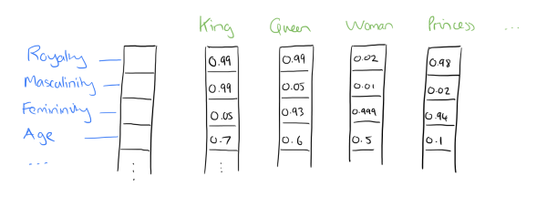
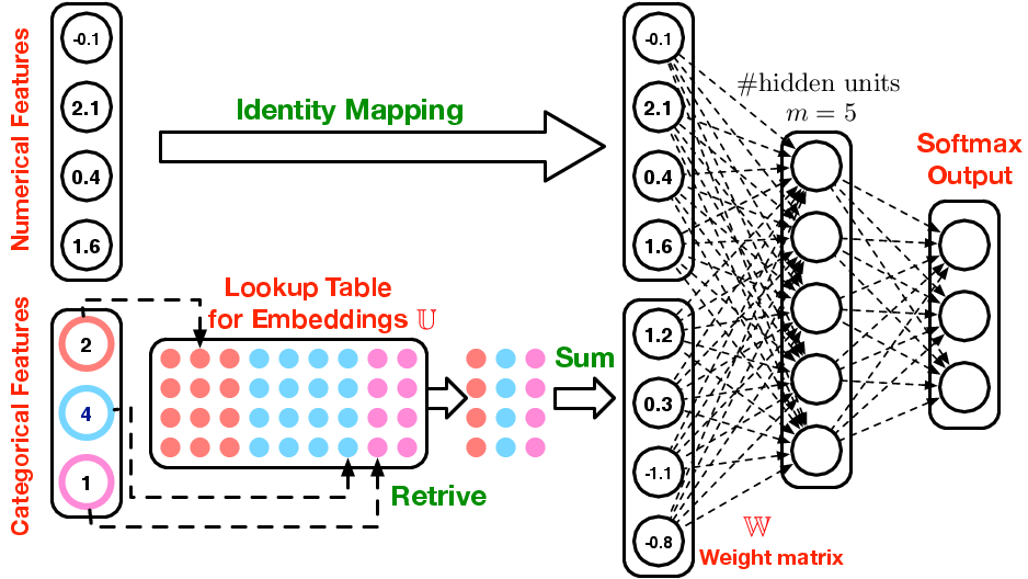
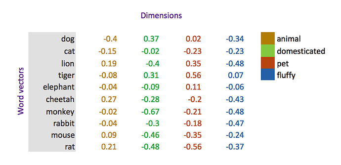
If we treat something as a category, we will be giving it an embedding matrix. We will essentially be developing a description vector. If its continuous, we need to find a underlying function that relates to it. Words easily fall into this categorical.
Some more examples of embeddings. Note that these different color categories are arbitrary and must be interpretted after the fact. The dimension (how many colors, or royalty etc. ) must be chosen beforehand and trained on a deep learning

How do you deal with dates?Turning day of the week data into an embedding
Proximity to holiday. Either upcoming or previous.
- How long has it been since the last promotion?
- How long till the next promotion?
def get_elapsed(fld, pre):
    day1 = np.timedelta64(1, 'D')
    last_date = np.datetime64()
    last_store = 0
    res = []

    for s,v,d in zip(df.Store.values,df[fld].values, df.Date.values):
        if s != last_store:
            last_date = np.datetime64()
            last_store = s
        if v: last_date = d
        res.append(((d-last_date).astype('timedelta64[D]') / day1).astype(int))
    df[pre+fld] = res
Using the function for state holiday and school holiday
fld = 'SchoolHoliday'
df = df.sort_values(['Store', 'Date'])
get_elapsed(fld, 'After')
df = df.sort_values(['Store', 'Date'], ascending=[True, False])
get_elapsed(fld, 'Before')
fld = 'StateHoliday'
df = df.sort_values(['Store', 'Date'])
get_elapsed(fld, 'After')
df = df.sort_values(['Store', 'Date'], ascending=[True, False])
get_elapsed(fld, 'Before')
Moving Averages (take a 7 day period … create a rolling sum) AKA window functions
bwd = df[['Store']+columns].sort_index().groupby("Store").rolling(7, min_periods=1).sum()


