Thinking that understanding the basic theory about Naive Bayes would help understanding lesson 5, and I happened to present a paper about sentiment classification on the Business Communication class, I humbly want to share part of my presentation on using Naive Bayes Classifier to classify sentiment of movie reviews. I am too lazy to transform all the formulas into markdown so I just take the screen-shot of my word document. The complete version of my presentation which includes maximum entropy and support vector machine classifier is also attached. Hope it helps.
Many thanks for sharing. I do think that you could create a terrific blog post based on your presentation combined with what we learned in the naive bayes lesson - some students in the DL class are saying they found this lesson particularly challenging, so I think it could be quite a popular article when the MOOC comes out.
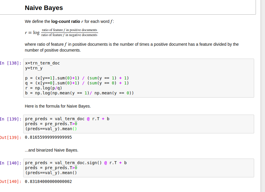
Hi , I was wondering if there might be a miscalculation with Naive Bayes in lesson 5 nlp notebook ? I tried out what I think as the right way to do it following the steps in excel spreadsheet and I’ve noticed a slight improvement (since calculations are deterministic it might be worth noticing).
Again, I am also not a fan of paying very much attention to Naive Bayes compared to embeddings or RNNs but still it’s good to know the intuition of it. Please correct if I am thinking wrong with calculation (code) changes.
Another thing I don’t know whether if it’s only me but BOW_Dataset was missing attribute X when I tried to fit learner (btw my fastai is up-to date), so I’ve noticed self.X was missing, changed it like this:
class BOW_Dataset(Dataset):
def init(self, bow, y, max_len):
self.bow,self.max_len = bow,max_len
self.c = int(y.max())+1
self.n,self.vocab_size = bow.shape
self.y = one_hot(y,self.c).astype(np.float32)
x = self.bow.sign() self.X = x
self.r = np.stack([calc_r(i, x, y).A1 for i in range(self.c)]).T
Hi Kerem, I also noticed the difference between the code and Excel spreadsheet. In the Excel spreadsheet, the ratio of feature f giving a positive label is calculated as the number of a feature in all positive documents/the number of positive documents; however, in the code, it is calculated as the number of a feature in all positive documents/ the number of all features in all positive documents. The latter one conforms to the theory of Naive Bayes, though in practice it might not have better accuracy or even worse as you indicate.
(Hey @parrt, what’s the correct way for me to report an infraction of the secret Rule Zero of the academic honor code: “no student will make his teacher look stupid by pointing out their incompetence” ?)
Please correct me if wrong, but the way I am seeing Naive Bayes, the code looks fine. i.e. p should be equal to number of a feature in all positive documents/ the number of all features in all positive documents.NOTnumber of a feature in all positive documents/the number of positive documents.
I tried to read it in below links and still thinking p,q to be divided by total number of all words in class A. not total number of documents. Don’t know why accuracy increased.
Although b seems to be right to be updated to something like b = np.log((y==1).sum()/(y==0).sum())
Sorry!
But the way you had shown in lecture, it was number of a feature in all positive documents/the number of positive documents., the thing that Kerem is saying. But code is in line with what’s there in paper. So yeah, there is a difference in excel file and code. Not sure which one is right. (imho what’s there in code and paper)
OK I’m not sure I’m thinking that clearly ATM, but here’s what I think is going on:
The Excel version only makes sense as a probability when used with binarized features. The probabilities are calculating the proportion of documents in a class that have the word w
The python version works for both binarized and raw features. It calculates the proportion of words in a class that are word w
I wrote the Excel version without looking up any references but just using (what I thought was) common sense. The python one I wrote months ago, and think I actually worked from a reference book. As @groverpr says, the python one appears to be more in line with the generally accepted approach.
However my Excel “common sense” approach makes more intuitive sense to me. It’s interesting that @kcturgutlu shows it’s actually better. (Although when used as a feature in the logistic regression it ends up identical, FYI).
Does this analysis seem about right? Has anyone come across materials that show something more like my Excel approach?