<<< Post: revisão | Post: Lição 6 >>>
(conteúdo do post “Wiki: Lesson 5”)
Lesson resources
Links to more info
Other datasets available
Video timeline
-
00:00:01 Review of students articles and works
-
00:07:45 Starting the 2nd half of the course: what’s next ?
MovieLens dataset: build an effective collaborative filtering model from scratch
-
00:12:15 Why a matrix factorization and not a neural net ?
Using Excel solver for Gradient Descent ‘GRG Nonlinear’
-
00:23:15 What are the negative values for ‘movieid’ & ‘userid’, and more student questions
-
00:26:00 Collaborative filtering notebook, ‘n_factors=’, ‘CollabFilterDataset.from_csv’
-
00:34:05 Dot Product example in PyTorch, module ‘DotProduct()’
-
00:41:45 Class ‘EmbeddingDot()’
-
00:47:05 Kaiming He Initialization (via DeepGrid),
sticking an underscore ‘_’ in PyTorch, ‘ColumnarModelData.from_data_frame()’, ‘optim.SGD()’
-
Pause
-
00:58:30 ‘fit()’ in ‘model.py’ walk-through
-
01:00:30 Improving the MovieLens model in Excel again,
adding a constant for movies and users called “a bias”
-
01:02:30 Function ‘get_emb(ni, nf)’ and Class ‘EmbeddingDotBias(nn.Module)’, ‘.squeeze()’ for broadcasting in PyTorch
-
01:06:45 Squeashing the ratings between 1 and 5, with Sigmoid function
-
01:12:30 What happened in the Netflix prize, looking at ‘column_data.py’ module and ‘get_learner()’
-
01:17:15 Creating a Neural Net version “of all this”, using the ‘movielens_emb’ tab in our Excel file, the “Mini net” section in ‘lesson5-movielens.ipynb’
-
01:33:15 What is happening inside the “Training Loop”, what the optimizer ‘optim.SGD()’ and ‘momentum=’ do, spreadsheet ‘graddesc.xlsm’ basic tab
-
01:41:15 “You don’t need to learn how to calculate derivates & integrals, but you need to learn how to think about the spatially”, the ‘chain rule’, ‘jacobian’ & ‘hessian’
-
01:53:45 Spreadsheet ‘Momentum’ tab
-
01:59:05 Spreasheet ‘Adam’ tab
-
02:12:01 Beyond Dropout: ‘Weight-decay’ or L2 regularization
1 Like
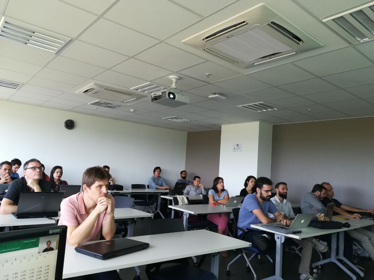
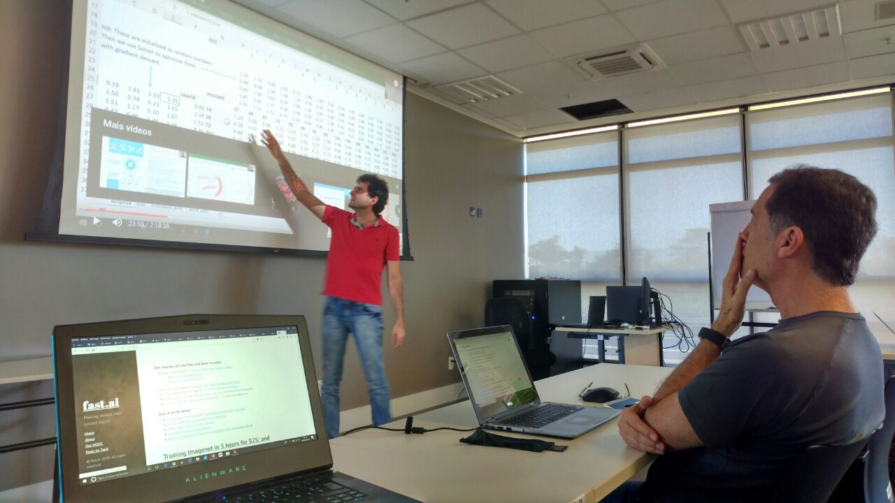
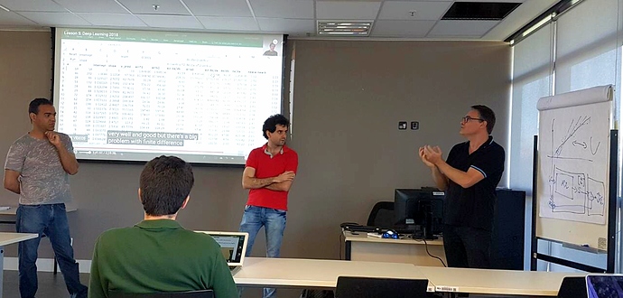
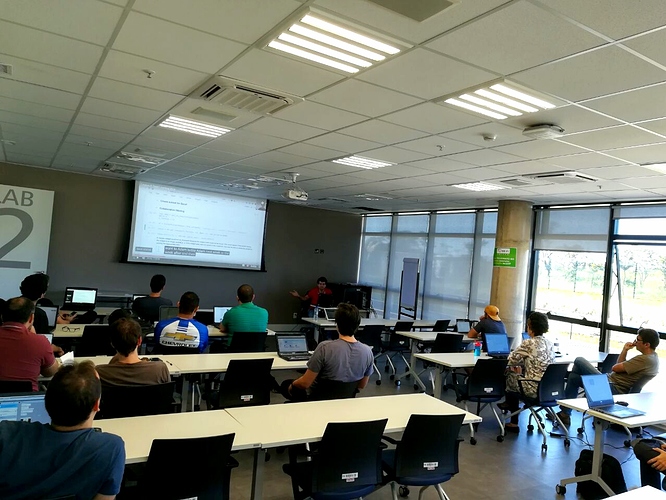
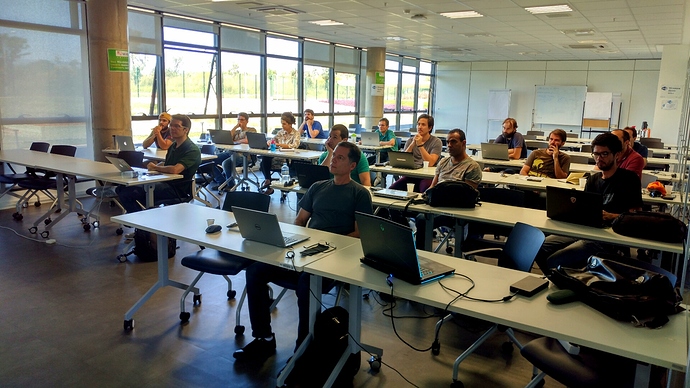
As fotos da turma de sábado 05/05/2018 com instrutor João Ferreira 
1 Like
Hoje de manhã, falei que os vetores de embeddings são necessários no PLN para traduzir/veicular o sentido de cada palavra em relação ao corpus : é verdade.
No entanto, falei após que uma imagem não precisa de vetores de embeddings porque um pixel tem só um valor (que não é o caso de uma palavra). Minha afirmação era falsa por metade 
Com certeza, o valor de um pixel tem somente… um valor mas o mesmo objeto numa imagem pode ter sentidos diferentes. Por exemplo, a luz verde or vermelho de um táxi pode significar que ele esteja livre ou ocupado.
E ai, se um pixel não precisa de um vetor de embedding, uma imagem (um conjunto de pixels) sim, no caso de uma classificação que precisa fazer a diferença entre vários estados de um mesmo produto (e para evitar classificar da forma tradicional todas as possibilidades com um CNN…).
Assista a este video para entender esse caso :
OHE * weight matrix == embedding
From @jeremy (link to post) :
Why do we use Collaborative Filtering models ?
From “Various Implementations of Collaborative Filtering” 
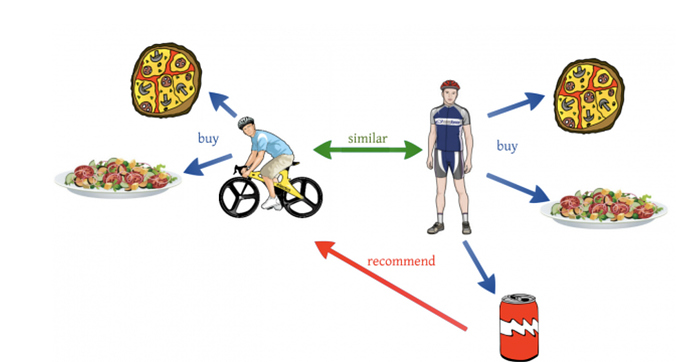
We see the use of recommendation systems all around us. These systems are personalizing our web experience, telling us what to buy (Amazon), which movies to watch (Netflix), whom to be friends with (Facebook), which songs to listen (Spotify) etc. These recommendation systems leverage our shopping/ watching/ listening patterns and predict what we could like in future based on our behavior patterns. The most basic models for recommendations systems are collaborative filtering models which are based on assumption that people like things similar to other things they like, and things that are liked by other people with similar taste.
Verifique a sua compreensão da lição 5
<<< Verifique a sua compreensão da lição 4 | Verifique a sua compreensão da lição 6 >>>
Oi pessoal,
Eu assisti novamente ao video da lição 5 (parte 1) para melhorar meu entendimento dela e tomei notas do vocabulário usado pelo @jeremy.
Vamos jogar um pouquinho ! Concorda ? 
Você pode dar uma definição / uma URL / uma explicação para todos os termos e expressões a seguir?
Se sim, você entendeu perfeitamente a quinta lição! 


PS: se você não quiser se testar ou se quiser checar as suas respostas, vá para o post “Deep Learning 2: Part 1 Lesson 5” do blog de @hiromi : " super travail !!! " 
-
Structured Deep Learning : not a lot of paper on Deep Learning for structured data with comparaison to computer visionand language natural
- Towards Data Science
- Kaggle competition : Plant seedings Classification
- this course starts the 2nd half of parte 1 (let’s dive into the source code) : the first half was about understanding the concepts, knowing best pratices and running the code by going through aplications (notebooks); this one is about the code to write with a high level of description
-
Goal of the lesson : create a collaborative filtering model from scratch (notebook : lesson5-movielens.ipynb)
- Movielens dataset is a list of ratings
- we use userid and movieid (categorical variables) and rating (independant variable) (we do not use here timestamp)
- we get the users that watch the most movies and the movies most watched
- in the beginning of the course, we are not going to build a Neural Network but a collaborative filtering model.
- we use pandas in the jupyter notebook in order to create a crosstab table of the 15 users they give the most ratings vs the movies which were the most rated
- Then, we copy/call this table of numbers atuais in Excel.
** functions to know : pd.read_csv, groupby(), sort_values(), join, crosstab()
** We copy/paste the stucture of the table and put ratings numbers by random (how ? each rating is the dot product of 2 vectors : one that qualifies a user and the other that qualifies a movie. The initial values of these 2 vectores are taken by random. When there is not a true rating, we put zero as the prevision).
** Then, we create an error cell that computes the root-mean-square error (RMSE) which is square root of the mean of the error square).
** This is not a neural net but a single matrix multiplication between 2 matrixes (one of the users and one of the movies)
** In Excel, we can do Gradient Descent : go to Data >> Solver >> Objective function (the cell with the RMSE) : cells to change + MIN (using GRG NonLinear which is Gradient Descent method)
** As this is not a Deep Neural Network (there is no hidden layer), we call this shallow learning.
** We do here a matrix decomposition (probabilistic matrix factorization)
** The numbers for each movie and for each user are called latent factors do vector de embeddings. The gradient descent tries to find these numbers.
** how do decide the dimensionality of our embedding matrix ? No idea. We have to try things and this have to represent the true complexity of the system but not too big (avoid overfitting, avoid time consuming for computation)
** the negative value in the embedding matrix represents the oposite (ie, I do not like)
** if you have a new user, you must retrain your model but we will see that later
- Back to the jupyter notebook
** we use get_cv_idxs() to get our validation set
** wd means weight decay (L2 regularisation)
** n_factores : size of our embedding matrix
** our data model is cf = CollabFilterDataset.from_csv()
** our learn model is learn = cf.get_learner() with an optimizer which is optim.Adam
** learn.fit(lr, wd=wd, cycle_len = 1, cycle_mult=2)
** the error is the MSE (mean squared error), not the RMSE, then we need to take the root
** that’s all : the fastai library allows us to get a better validation loss in 3 lines of codes (cf, learn, learn.fit) than the actual benchmark
** Let’s try now to build the Collaborative Filtering from scratch using pytorch
** we can create a torch Tensor in pytorch by using capital T : T([1.,2],[3, 4])
** The multiplication of 2 torch Tensor is a element wise multiplication
- we are going to build a layer (our custom neural net layer or custom pytorch layer) = a pytorch module
** And then we can instantiate a model as a pytorch module, use it as a function that we can compose with very conveniently (take the derivative for example)
** to create a pytorch module, we need first to create a pytorch class in which you return the calculated value in a special method called forward
** in a neural net, when you calculate the next activations, it is called the forward pass : it is doing a forward calculation (the gradient is called the backward calculation but we do not have to define that as pytorch does it automatically)
** first thing to do is to get a continuous index of userid and movieid to avoid a huge embedding matrix (we use for that the unique() method and the creation of dictionary)
** each time we want to pass our new number of users, movies (we call them states), we need a constructor for our class (this is a special method def __init__)
** 2 other things to get a full pytorch layer : we inherit of the nn.Module class to get all cool staff from pytorch and we need to call the super class constructor (when we create our own constructor : super().__init__())
- Then, we need to give some behavior and we do that by storing somethings in it.
** we create self.u which is an embedding layer : self.u = nn.Embedding(n_users,n_factors), same thing with movies
** we need now to initialize by random our embedding matrices but with small numbers
** the embedding matrix is not a tensor, it is a variable (a variable is a tensor and it does automatic diferentiation)
** then to get the tensor, we use the data attribute
** uniform_ does operate in the same tensor (fill in the matrix)
** finally, we create the forward method by grabbing the embeddings vector for the user and the movie (minibatch of them : this is done autmatically by pytorch : DON’T DO A FOR LOOP because it does not use GPU), and return the dot vector multiplication
** Then, we can write our 3 lines of codes : data with the fastai library, our pytorch module (our model) that we initiate with our EmbeddingDot class, and finally we can fit our model by using the pytorch way
-
Biais
** we need to add a constant for each user and one for each movie to take account the fact that for example the user always gives a high rating and that a movie is liked by everyone because these are biais : they hide the true diferences.
** Then, we modificate our pytorch module to take account the biais.
** we use broadcasting to add a matrix and a vector (squeeze())
** then, we use a sigmoid function to put all calculations between 1 and 5 (it is not common but help)
** all the functions in pytorch are availables in capital F (F.sigmoid)
** we must precise cuda() as we don’t use a learner from fastai
** One remark : we do not do exactly matrix factorization
** before the Netflix prize, this matrix factorization had actually already been invented but nobody noticed and in the first year of the Netflix price, someone wrote this really famous blog post where they basically said “eh just use it” (2009 by BellKor’s Pragmatic Chaos team)
- let’s create a neural net version of this
** A one embedding is exactly the same as doing a one hot encoding.
** An embedding is a matrix product
** the only reason it exists, it is because it is an optimization : it is a computational performance thing for a particular kind of matrix multiplier
** Our neural net will take in the entry a concatenation of the 2 embeddings vectores : this is an embedding net
** We start with 2 linear layers (then the first one is an hidden layer) and the second one has only one output as we want a single number (we use nn.Linear()). These layers are Fully Connected Layers.
** In the forward method, we grab the data (users and movies) and create the embeddings vectors, we concatenate theses vectors with torch.cat(), we add dropout, we add relu on activations of the layer 1 (F.relu), and activation function after the layer 2 (F.sigmoid())
** Then, we create our data model, our learn object and we fit this learn object with the MSE function (F.mse_loss)
** Point important : we do not need to get the same size of latent factors in the embeddings vetores of user and movie (for example, the embedding vector of the movies can have latent factors for genre and duration for example besides the n_factors shared with the user embedding vector)
- Let’s use graddesc.xlsm to implement Gradient descent in excel
** errb1 : finding the derivative through fine diferencing
** derivative of the cost function is how the dependent variable (loss function) changes when the independant variable (intercept or slope) changes
** Jacobian and Hessian matrix
** Chain rule
** mini batch de size 1 = online gradient descent
** problem : it takes time and more, we can see that the error function goes down the same way : it means we can go faster. This is momentum
- momemtum is a linear interpoletion between our derivative of the error function (small number) and the ones calculated before : keep doing the way we did before and upgrade a little bit
** everyone uses momentum
** More one point : in momemtum, the learning rate does not change
-
Adam
** We use SGD with momentum by default in the fastai library but we can now use Adam with weight decay in Fastai (Adam-W)
** Adam has 2 parts : one uses the momemtum of the gradient and the other part uses the momentum of the gradient square
** we use a lot the linear interpolation in DL papers
** if there is a lot of variance of the gradients, the number that divises the learning rate (the square root of the moving average of our squared gradient) will be high and than, the learning rate general is low
** ADAM is finally an adaptative learning rate (but there is only one learning rate)
-
L2 or weight decay
** when you have huge neural network, lots of parameters, more parameters than data points : then, regularization is important (like dropout)
** we take our loss function and add an aditional piece to that (square of the weights)
** the loss function wants to get the weights small
** if you have a huge weight decay, the gradient descent will keep your parameters to zero : it will never overfit
** if you then decrease the weight decay, some parameters will rise but the ones useless will stay to zero (proche de zero)
** when there are a lot of variation, we end up decreasing the amount of weight decay (and the oposite is true)
-
ADAMW
** penalize paremeters with weight very high unless their gradient varies a lot : but we do not want that
** so in ADAMW we do not mix weight decay with ADAM
** majority of models uses dropout and weight decay
