Hi Everyone,
I am trying to understand the paper reading for lecture 8, so I went to this blogging site which was even mentioned in Lesson 8, I am still unable to understand the concepts. The is the link of the blog is https://pouannes.github.io/blog/initialization/
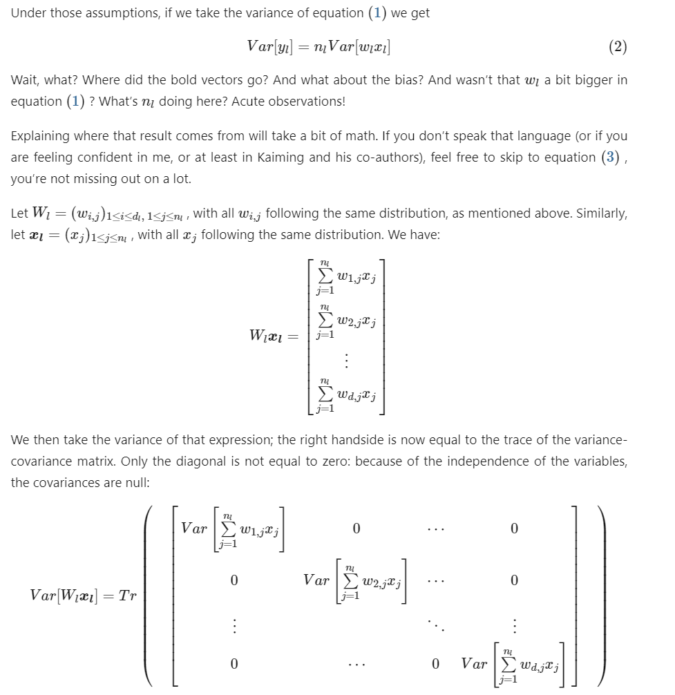
And I am unable to understand this second equation in the image below, even though how the paper arrives at this is also mentioned. Can anyone help me understand it or direct me to an easier blog?
@karanchhabra99
I’ll give you an intuitive answer to your question, hopefully it won’t trouble you then.
The authors defines
\mathbf{y}_{l} = \mathbf{W}_{l}\cdot \mathbf{x}_{l}
Which is essentially the sum of all products from the matrices W and x. The sum contains n_{l} elements in all.
Now a single element of the sum is w_{l} \cdot x_{l}. I think it is clear that when n_{l} such terms are added up, what we get is an element of the column matrix \mathbf{y}_{l} , or y_{l} .
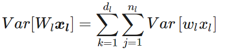
Now, what is variance? Variance is the measure of how spread out the distribution is. The sum of products \mathbf{W}_{l}\cdot \mathbf{x}_{l} is a distribution. Each w_{l} \cdot x_{l} is a part of this distribution. And this w_{l} \cdot x_{l} has its own variance, equal to Var(w_{l} \cdot x_{l}) .
n_{l} such elements spread out the distribution, and so the sum of n_{l} independent distributions have a n_{l} times bigger distribution (in terms of how much it is spread out).
So that’s how Var[y_{l}] = n_{l}Var(W_{l}\cdot x_{l}) . Hope that clears things out.
This is exactly what is done in the blog you mentioned, just below equation 2.
Thank @PalaashAgrawal
That is really helpful