I set up a Gradient account on Paperspace, and imported the Fast.AI notebook for the course. Lesson 2 does not work by default, as it is missing the Planet dataset; there do not appear to be instructions in the notebook as to how to import the dataset. What’s the easiest way to import the data?
Answered my own question by searching the Wiki, a lovely walkthrough written bt daphn3cor. Perfect for learning how to install files under the Gradient Jupyter notebook on Paperspace.
Thank you for spending time to provide this for newcomers; I would have gotten stuck without this information.
How does batch size impact image augmentation and model performance? My understanding is that in one epoch with augmentation, the network is trained on one augmented version of each image in the dataset. Batch size affects the number of iterations/weight updates within an epoch. Larger batch sizes require more epochs to converge because each epoch has fewer weight updates compared to epochs with smaller batch sizes.
If I use a large batch size, does that mean the network is seeing more images per weight update? In the context of using image augmentation to expand a limited dataset, would a higher batch size be advantageous because the network would see more augmented versions of images over the course of the training process?
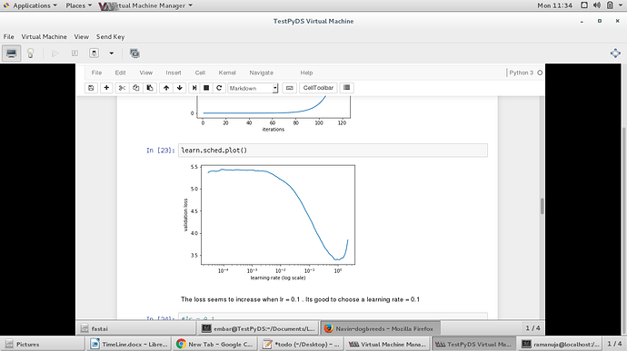
My guess is that you started from an already trained model. Thus you don’t see any decline in loss. As I understand it, for lr_find() to work, you’ll have to start from untrained (or only slightly trained) model.
Question about Lesson 1 task: test/validation score and accuracy given in Lesson 2 video
I have a problem understanding why training loss is bigger than validation loss function (see 4:13 in the video of lesson 2). As far as my understanding goes, training loss will almost always be smaller than validation loss (if we don’t count occasional lucky chance). After all, training data is what we see.
Second question is about accuracy we can get. Please take a look at accuracy of the model with augmentation at 25:44 in the video of lesson 2. The value of 0.936 is quite high and I would like to hear about accuracy you get at this point. If I run this few lines of code multiple times, I get accuracy all over the place, so is this the reason for quite high accuracy in the video?
Histogram of the accuracy of the above code:
I know one of the method for getting better model is to retrain the model from different starting position, so this might be one reason. Quite oddly, I get somewhat different histogram if I don’t remove folders models and tmp (although this is a subjective conclusion, with 100 runs only).
Hi GregFet: May you share the link on Kaggle to download the satellite dataset? Thanks a lot.
So in the lesson Jeremy mentioned that the validation images are center cropped to be square. But are the training images also cropped that way? It seems to me it would be the case, but that’s not clear.
Hi all, i tried building an image classifier based the steps outlined in the lesson 1 notebook.
I wrote my first medium post based on the results i had, please check it out and let me know your thoughts
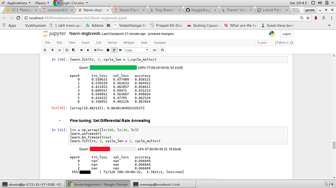
I was doing the dog breeds identification in AWS . I was getting Nan in the training & validation loss while training with differential learning rates.
attached the image
I was using learning rate = 0.2
May I know why it happens.
I have the same question. How is the model handling variable input sizes?
My notebook is similar to Jeremy’s dogbreeds notebook shown in the video except the below:
-
learning rate: Mine Jeremy
0.2 1e-2 -
Arch : resnet34 resent50
Later when I changed the learning rate to 1e-2 the Nan’s observed in the training/validation loss disappeared.
Is it that Nan’s appear when the learning rate is much higher as in this case 0.2 or 0.1 ?
The lr_finder was showing that lr of 0.1 would be a good choice…
Since no one answered, I’d add what I’ve found in case it’s helpful to someone: the code is buried deep in the transforms.py of the fast.ai library. By the code, the cropping of the validation images depend on the cropping of the training images. If the training images are cropped in the “random” or “googlenet” way, then the validation images are centre-cropped; otherwise, the validation images are cropped the same way as the training images.
Guys can anyone tell where to find all trained model weights by jeremy in lectures as i don’t have sufficient computational resources to train which is demotivating as i am not able to see results on my pc of the models which we are making.
This is a non-answer
how did you resolve this?
Having some issues with overfitting on the dog breeds challenge. I walked through the code as Jeremy explained his process but as soon as the first learn.fit(1e-2,5), my results diverge from his.
epoch trn_loss val_loss accuracy
0 0.536105 0.319523 0.902153
1 0.350298 0.297175 0.902642
2 0.254736 0.266593 0.912427
3 0.19815 0.265514 0.91683
4 0.166361 0.253992 0.918297
as you can see, my trn_loss rapidly decreases below the level of val_loss. As I move through the exercise, my trn_loss continues to drop while val_loss maintains at ~0.23-0.25.
I believe I’m overfitting, but i’m confused how this could happen if I’m running ostensibly the same code as Jeremy. The only change I had to make was to the batch size (decreased to 20) because I was running into cuda memory error. Could this cause this issue?
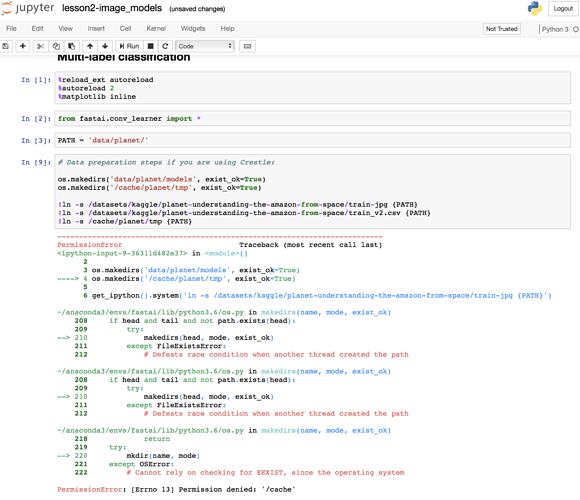
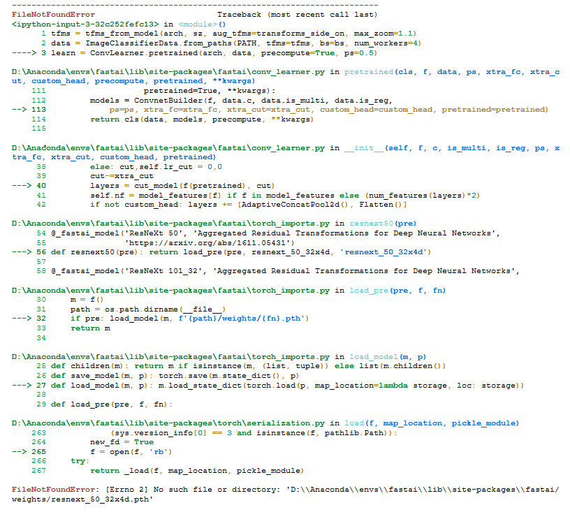
Hi to everyone! Please, help me with some error with notebook lesson2 “Multi-label classification”.
I am using a paperspace, so run cell. Below is the error.
thanks in advance.
Hi @cqfd , I have a doubt regarding “pre_compute” . It is mentioned that we pass in that dataset once (without any data augmentations) to get the activation vectors of each image. But when we go to the code,
Initially, in #1, It is written that pre_compute=True, and then in the next step we do
1.learn.fit(.01,1), doesn’t this mean that the weights of resnet34 arch are getting updated?
- For data augmentation, we put “pre_compute=False” for not computing activation vectors for data augmented images and do “.fit” again. My question is, how do you get activation vector for a rotated image which is diff from actual image. Do we use activation vectors of the original image? Are we passing the rotated image through resnet arch? If yes, that means we are computing activation vectors which goes against pre_compute=False?
I’m slightly confused about points 5.-7.:
Review: easy steps to train a world-class image classifier
- precompute=True
- Use lr_find() to find highest learning rate where loss is still clearly improving
- Train last layer from precomputed activations for 1-2 epochs
- Train last layer with data augmentation (i.e. precompute=False) for 2-3 epochs with cycle_len=1
- Unfreeze all layers
- Set earlier layers to 3x-10x lower learning rate than next higher layer
- Use lr_find() again
- Train full network with cycle_mult=2 until over-fitting
Let’s say that for step 4., I do:
learn.precompute=False
learn.fit(lrs=1e-2, n_cycle=3, cycle_len=1)
If after that, I do
learn.unfreeze()
lrf = learn.lr_find()
learn.sched.plot()
then the learning rate finder will show me the loss as a function of learning rate, assuming that I use the same learning rate for all layers However, what I’ll actually do is use differential learning rates, like lrs = np.array([1e-4,1e-3,1e-2]).
So my question is: Can I tell the learning rate finder to show me the loss as a function of late-layer learning rate, assuming that early/middle-layer learning rate is 100/10 times lower than late-layer learning rate?


