The loss seems to go down super fast at the beginning, but stays around 676 at the end rather than approaching 0, even when I ran apply_step(params) 20 more times. The graph of the predictions also does not match the original graph even after lots of training. This seems to be different from the 2019 course, where the linear regression was able to match the original data almost perfectly. Why is this?
@stonecr0wn
If you look at the data you’re trying to fit, you’ll see that it doesn’t Exactly follow quadratic distribution - there’s some noise in the data! And so if you try fitting a quadratic function through the data, you’ll never be able to cross the function through all the points. That’s usually true in data science - the data you’re given follows some general trend, but there is always some noise. We’re usually interested in finding the general trend, which is, in this case, a quadratic distribution. We would like to find the quadratic equation that “Best” fits the distribution. You’ll never be able to fit the distribution perfectly, with this function.
Hope this helps!
Getting a loss of 0 (or really close to it) is actually indicative of an important problem in machine learning: overfitting.
If the loss is 0, it means the neural network has perfectly learned the training data. But we don’t really want it to memorize the training data. We only want the model to learn interesting patterns from the data, so that we can detect those same patterns in other, unseen data too.
With a loss of 0, your model may have learned the wrong thing. It has a perfect score on the training data. But will it work OK on new data too?
The actual value of the loss is not important. We just want it to go down over time, so we know the model is learning something. But we need other tools to determine if the model has learned the correct thing (validation metrics).
In order to improve the fitting, it is best to expand the time interval from 0…20 to -20…20. So the code needs to be updated as follows:
time = torch.arange(-20, 20)
speed = torch.randn(40)3 + 0.75(time-9.5)**2.0 + 1
My guess is that, in this way, the SGD algorithm has a better “understanding” of how the quadratic function behaves for inputs below 0, and then has a better chance to optimally update the parameters (especially for time values near 0).
Secondly, you need to increase the number of steps. If you use 500,000 steps, you will see the loss function going down to 8.6.
I just noticed this issue. It’s because the guessed equation is bad! a*x**2 + b*x + c can never approximate that curve well. That function will always have a zero value at x=0.
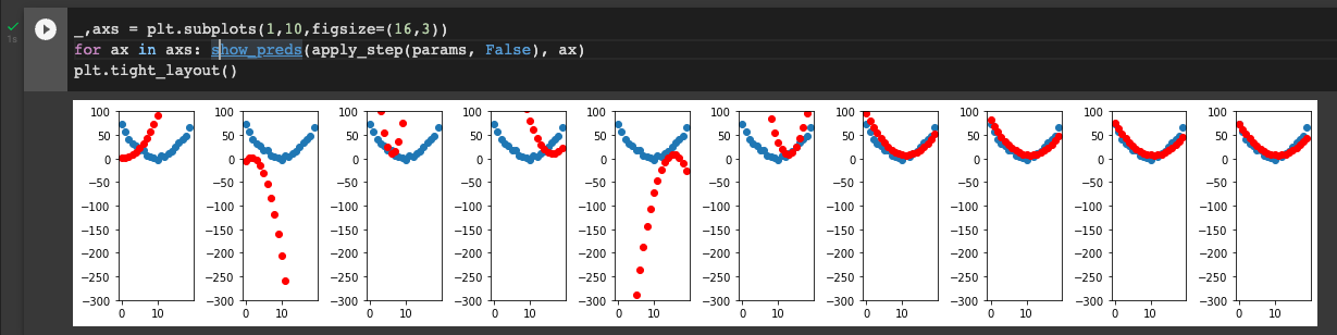
I added one more parameter and got a much better fit: a*(x-d)**2 + b*x + c.
Here’s the more satisfying output with this change and going for only 10 steps, and a learning rate of 1e-4:
Notice something funny here: d (effectively the x offset, where the parabola hits a zero derivative) oscillates around the correct value from left to right and back to the center.