Why do we need the unconditioned embedding?

[dpoulopoulos (Dimitris Poulopoulos)]

In the Stable Diffusion deep dive notebook, I see that we create a set of embeddings: one for our prompt and one unconditioned, meaning an embedding for the empty prompt. Then, we concatenate these two in a new text embedding tensor, which we pass to the Unet as it predicts the noise residual.

The idea is to use the result to provide guidance, and push our model toward generating images that are closer to the prompt we passed:

# perform guidance
noise_pred_uncond, noise_pred_text = noise_pred.chunk(2)
noise_pred = noise_pred_uncond + guidance_scale * (noise_pred_text - noise_pred_uncond)

But why do we need this? Why don’t we just encode our prompt and use only that. Why do we need the unconditioned embedding?

[bipin]

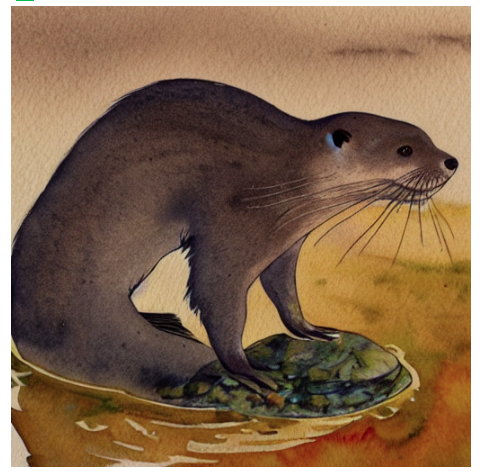
At 30 iterations, the image generated by the model is worse when only using prompt embedding(1st image) while it gives better image when using prompt and unconditioned embdedding(2nd image):

So I think the randomness helps the model generate better images faster.

[pcuenq (Pedro Cuenca)]

I think the conceptual idea goes something like this:

• Generate an image without text conditioning. This will make the model move in a random direction so any type of image can be generated.
• Generate an image with text conditioning. The model will try to find some image that resembles the text we used.
• Consider the vector between the unconditioned and the conditioned images. Move further away in that direction (as far away as dictated by the guidance_scale parameter).
• Use that point as the reference for the next step.

So there are two generation processes running in parallel. In practice, the latents for both the unconditional and the conditioned texts are concatenated so we can perform a single forward pass instead of two.

[barnacl (Rekil Prashanth)]

Adding to what @bipin & @pcuenq have mentioned:
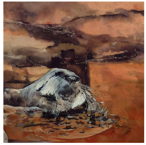
if you use the prompt + random noise and no unconditioning you end up with some thing that kinda looks like an otter:

Now if you use the unconditioned scenario where you have no text (actually the model is using a start of text token and a bunch of end of text tokens to represent this) and we use the same random noise that we used to generate the image with the prompt in the above case it gives us a random image

Now we used the same random noise to generate these images the text prompts were different. So if we subtract them we cancel out the effect of the random noise and keep the direction of the difference of text. Then when we multiply this by the guidance_scale, we are moving more in the direction of the prompt - “A watercolor painting of an otter” .
So i was wondering what if we take the same random noise but a different prompt (a prompt that should be very different from the stuff you are trying to generate) say -“solar system with 9 planets”. Now if we subtract them and use guidance_scale as before we get:

Here is the colab notebook if you want to play around with (my explanations may be wrong but it’s fun to play around. Add your insights too, there is some stuff about scheduling guidance_scale, as we get closer to the final image we probably want to reduce thee guidance_scale etc)

[akash5474 (Akash)]

It looks like there are two parts to this question. The first part, why are the embeddings concatenated and passed together? I believe this is so we can use our unet to make two predictions at the same time in one forward pass (with batch_size of 2 from torch.cat) instead of making the predictions one by one.

For the other part, why do we need the unconditional embedding? This is how I’m understanding it currently:

The noise_pred_uncond gives us a baseline. When our model sees the noised input without a prompt, it makes a guess which we can expect will be less like our desired outcome since it doesn’t have the prompt to help. An analogy would be like you asking a friend to draw what your are imagining in your head without giving them any more information. Your friend might draw something good or interesting, but the drawing will very likely not be anything like what you’re imagining.

The noise_pred_text is the prediction when our model also has a hint (the prompt) so we would expect this prediction to be closer to our desired outcome. It’s as if you were to instead ask your friend to draw what you are imagining in your head and including the hint “a watercolor painting of an otter”. The result might not be perfectly as you imagined, but it will be a lot closer.

By subtracting the noise predictions we get to know which variables have the largest differences between the two. With this information we have a better idea of which variables from the random unconditional prediction need to change the most and what direction they need to change (similar to subtracting vectors) in order to make the predictions less like a wild random guess and more like our desired outcome/prompt. We scale it up by some amount (guidance_scale) to give those differences a larger influence.

Using the same analogy, it would be like telling your friend what to change (otter should look a little bit more cute, otter should be floating in the water facing up, etc.). You and your friend repeat the entire process a few times using the information obtained from the previous drawing. Eventually you should end up with a picture that looks closer to what you imagined.

Just for fun, with the prompt “a watercolor painting of an otter”, I switched the order of the subtraction which should mean we are guiding in the opposite direction away from the prompt:

noise_pred = noise_pred_uncond + guidance_scale * (noise_pred_uncond - noise_pred_text)

And this was the result:

[jeremy (Jeremy Howard)]

I do agree that picture is less like “a watercolor painting of an otter” than anything I could come up with!

[memetzgz (Maureen Metzger)]

I appreciate your explanation, it was really helpful.

Beginner question: I’m having trouble understanding why this can be done in one pass:

@pcuenq

So there are two generation processes running in parallel. In practice, the latents for both the unconditional and the conditioned texts are concatenated so we can perform a single forward pass instead of two.

How does the model know it’s generating two different images at the same time?

[pcuenq (Pedro Cuenca)]

@memetzgz

How does the model know it’s generating two different images at the same time?

If it was generating a single image without this trick, the batch size would be 1 and we’d do two passes. When we concatenate the embeddings, the batch size is 2 and we do one pass. (Same thing if the input was a batch with several images, we just double the batch size concatenating as many unconditioned embeddings as images in the batch).

This is the line of code where it happens, it might be helpful:

huggingface/diffusers/blob/main/src/diffusers/pipelines/stable_diffusion/pipeline_stable_diffusion.py#L276-L279

[memetzgz (Maureen Metzger)]

I knew I was missing something simple

Thanks, Pedro!

[jeremy (Jeremy Howard)]

Don’t forget to check out the blog post about this topic!:

Guidance: a cheat code for diffusion models

[ilovescience (Tanishq)]

This is needed for the classifier-free guidance (CFG). This is a super useful trick for improving conditioned diffusion models.

I know some folks have already given an explanation but thought I’d provide a different perspective.

First let’s think about classifier guidance. Here we use the gradient of a classifier to update our denoised image in a way that maximizes the correct classification. That looks something like this:

{\widetilde{\mathbf{\epsilon}}}_\theta\left(\mathbf{x}_t,\mathbf{c}\right)=\mathbf{\epsilon}_\theta\left(\mathbf{x}_t,\mathbf{c}\right)-w\sigma_t\nabla_{\mathbf{x}_t}\log{p\left(\mathbf{c}\right|}\mathbf{x}_t)

You can see the regular conditional noise predictor model and an additional term that is the gradient of the classifier with respect to the denoised image (w is the guidance scale, and \sigma is the noise variance from your schedule).

While this greatly improves the results over standard conditional models, the problem is this introduces the need for an additional classifier, one that actually needs to be trained specifically on these noisy images from the diffusion process.

So how could we overcome this? What if we could somehow construct a classifier from the generative model and use that for classifier guidance?

It turns out Bayes’ Rule gives us an expression for the classifier given other terms (here written in log where the multiplications/divisions become additions/subtractions):

\log{p}\left(\mathbf{c}\mid\mathbf{x}_t\right) = \log{p}\left(\mathbf{x}_t\mid\mathbf{c}\right)-\log{p}\left(\mathbf{x}_t\right)+\log{p}\left(\mathbf{c}\right)

The first term is your classifier (probability of class \mathbf{c} given \mathbf{x}_t), second term is the conditional model (\mathbf{x}_t given class \mathbf{c}), third term is the unconditional model (distribution of \mathbf{x}_t) and fourth term is distribution of the classes. We can plug this equation into classifier guidance. Since we are working with gradients with respect to \mathbf{c}, that last term drops out when we plug this into the classifier guidance, and simplifying we get:

{\widetilde{\mathbf{\epsilon}}}_\theta\left(\mathbf{x}_t,\mathbf{c}\right)=\left(1+w\right)\mathbf{\epsilon}_\theta\left(\mathbf{x}_t,\mathbf{c}\right)-w\mathbf{\epsilon}_\theta\left(\mathbf{x}_t\right)

So that’s the basic idea: constructing an implicit classifier from our combined conditional/unconditional generative model (which we represent with a single neural network) and use that for classifier-based guidance.

Jeremy already linked to the blog post I was going to link that goes into this in more detail