I was trying to reproduce the plots of the embeddings that @jeremy showed and I found that t-SNE has several parameters that can really affect the final visualization. I was wondering if you have some insights about the impact of different parameters and/or good practices. I attach my code (sorry. t’s quite nasty), for you to play too 
5 Likes
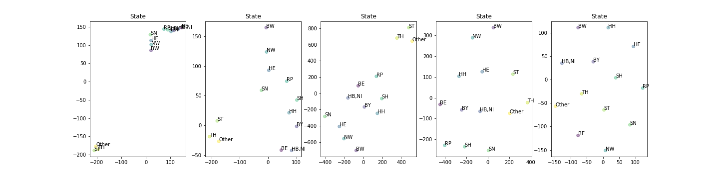
This first chart looks nice. What kind of t-SNE parameters you used to produce it ?
Perplexities = [2,4,5,10,25] (default is 30)
All the others are the scikit learn defaults:
early_exaggeration=12.0, learning_rate=200.0, n_iter=1000, n_iter_without_progress=300, min_grad_norm=1e-07, metric=’euclidean’, init=’random’, verbose=0, random_state=None, method=’barnes_hut’, angle=0.5
I played mainly with perplexity, early_exaggeration, learning_rate and angle.
First chart clearly displays 3 clusters and this kind of transformation one can effectively feed into kmeans.
I’ll see if I can find my tSNE notes / sources to confirm, but I seem to recall recommended Perplexities being in the 10-50 range (and having my most success in the 15-30 range, but this may be data specific).
I just googled around a bit and found this post which seems pretty on point to your questions:
3 Likes
I this case specifically you do have a ground truth. It is Germany’s states own topology.
Therefore in order to tune your TSNE representation you could conceivably calculate the discrepancy between your dimensionality-reduced embedding representations and the actual topology/map of Germany.
In pseudocode it would like something along these lines:
def calc_pair_wise_distances(topo): return [(from, to, dist) for i in topo]
def topology_ss(emb_topo, actual_topo):
pw_dist_emb = calc_pair_wise_distances(emb_topo)
pw_dist_actual = calc_pair_wise_distances(actual_topo)
squared_dist = [ (i[0][3] - i[1][3])**2 for i in zip(pw_dist_topo, pw_dist_actual)]
return squared_dist.sum()
Calculate that for all TSNE parameters and pick the combination with the lowest sum of squares