My understanding of backprop is that it’s an iterative approach of calculating partial derivatives. Let’s say we have f = mse(relu(x@w + b)). We can replace functions and say
u = x@w + b
v = relu(u)
z = mse(v)
As well, df/dx = df/dz * dz/dv * dv/du * du/dx. As we run backprop, after
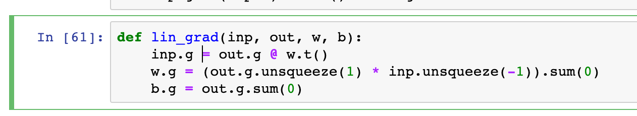
mse_grad, we will have inp.g = dz/dv, after relu_grad inp.g = dz/dv*dv/du and after lin_grad inp.g = dz/dv*dv/du*du/dx. Is anything wrong so far?
d/db
d(lin_grad)/db = 1 (vector). I get the part where we multiply that 1 with out.g, but why do we have to do .sum(0)? Is that because vector is broadcasted on dimension 0 when doing the forward pass?
d/dw
I do understand that we have to perform out.g(some_operation)x, but don’t fully understand whether it should be * or @. I know that I can’t do *, but I’d like to know some theoretical understanding instead of trying to make dimensions match.
d/dx
This component is completely unclear to me. My expectation is that it should be out.g(some_operation)*w.t. Again, I get that dimensions don’t allow that, but I’d like some theoretical understanding of why is that.
The reality is that the code in the notebook is an “optimised” version of the code. It makes sense to write it as is because it uses less memory and is faster, but definitely does not show how you’d calculate it step by step.
The paper linked explains how to calculate element by element of the result and then figuring out that it can be decomposed into a matrix multiplication.
Well, assuming that we have dz, we can work backwards. We know that x@w = z. dz has the same dimensions as z. we also know that each element in the first row of z was influenced by the first row of x. Hence w_{1,1}, a change in the first row, and the first column of w, will change the first row of dz, and the value of change is proportional to the first column of x, we need to sum up all the partial derivatives by the law of total derivatives. Hence dw = dz @ x.t I think this is the best and fastest way of thinking about these types of derivatives. Just look at one element of the matrix, in this case we took w_{1,1} and see a change on that which values of z will change.