Time series/ sequential data study group

[marvin (Marvin Hansen)]

@tcapelle

I understand that you want to predict future values based on past ones. There is a nice tutorial on getting started with time series with afocus on trends and correlation.

What I really need is to forecast the future of the Power, as accurate as possible for the near future, using the past values of P and the past and current values of T and time data.

To do so, I suggest conducting a correlation test whether there is a statistical significance between past and present values to determine whether you can use present values to predict future values.

The correlation coefficient of two variables captures how linearly related they are. If there-there is no (linear) relation between present and future values, how on earth can you make any useful prediction of future values? How do you know there is one?

A random walk dataset would have only a low correlation coefficient between the last and current value. That is exactly when you know that past values have no impact whatsoever on future ones. It is just random crap and no model in the world can predict that. To do a proper test, you add the (n) previous value of the target value to the feature set.

n = 1
X[“last_value-”+str(n)] = y.shift(n)

When you take a closer look at the RF Ada Boost model discussed in the tsfresh example, you noticed in the feature importance ranking that “feature_last_value” contributes to 88.5% of the accuracy while all the 347 features generated by tsfresh only added an accumulative 1.5% to the prediction.

Three insights:

1. You need to know the correlation coefficient between the past n values and the current value to figure out whether you are barking up the wrong tree.

2. To capture seasonality, cycles, and trend in time-series data, you need to categorify the date field. Jeremy made that abundantly clear in the lessons and also stresses it in the data preparation section of the Rossmann example

3. When adding tsfresh generated features, expect a 1 - 2% impact, as they demonstrated in the Google example. Turned out, many generated features suffer from low importance so ideally, you want to add correlated external data.

Hope that helps.

[muellerzr (Zachary Mueller)]

Hi all, I have been reading up on this thread as I am currently doing research with time series data. I’m wondering how best to split my data? It’s set up as 6 different events in 6 separate csv files and the goal is to identify what event it is given one column. I’m debating on a rolling-event style but I’m lost in how as each one has a sepearate time value which id like to ignore completely. I had very poor results with just a standard 80/20 random split (which would make sense as we are time trending data?) How would you recommend I select my ‘walk’ given the nature? Just do a walk with my validation being combined with all the events?

Thanks!

Zach

[akshayb7 (Akshay Bhardwaj)]

Hi everyone,
I’m fairly new to time-series analysis/prediction but have been asked to work on time-related live oil and gas data nonetheless. As a part of this, one of my first challenge is to remove unwanted noise from multiple data streams where most of them are related to each other, such that if we see a fluctuation in multiple of them at a time, then the data is valid but suppose if only one parameter fluctuates that is to be removed (kind of like a trend line I guess).
I have been trying to find methods to do so by searching for noise reduction/despiking techniques for multivariate data but haven’t had much luck in finding something useful. Does anyone have any tips on how to approach this problem?
I did look at techniques used in Human Activity Recognition models, but it wasn’t of much use.

While going through the forum, I saw @marcmuc has worked with energy related time-series previously, do you have any pointers sir?

P.S: Later I’ll have to use this cleaner version of data to make predictions for other datapoints and anomaly detection as well.

[marcmuc (Marc P. Rostock)]

Hi Akshay, there are many possiblilies in this area and it and depends very much on what your raw data is like and what you would like to achieve with it. It is also important to see, whether the data is supposed to be monitored in some “online fashion” as it is received, or whether you are doing analysis “offline” on historical data. But the prepping process for timeseries often is the most time consuming Dealing with missing values, with false zero values, detecting and removing false peaks/outliers, denoising, detrending. Regarding peaks if you know the bounds of your possible values exactly sometimes it is as easy as using hard thresholds, most often that doesn’t work though.

This is not a “solution” for you, but some suggestions of what you can look at regarding denoising / peak stuff and you can find some code here that you can test on your problem. Your solution will probably involve multiple steps and could use a combination of features gathered from these:

This kaggle kernel from the recent VSB Power Line competition shows nicely how denoising using DWT (discrete wavelet transforms) is done and aso shows high pass filtering. Results look like this:

This kernel from the same competition compares denoising by mean and denoising by Fast Fourier Transforms (FFT). Results:

A helpful metric wrt peaks is the “z-score”, these algorithms help you detect peaks when you have timeseries that are changing over time and you cannot use hard thresholds for peak detection by using rolling windows. Check out this helpful SO answer with a good explanation and links to implementations. The result looks something like this:

So you can detect peaks and then use this information in the next step (in your case use this output and then verify that this peak is present in “all” parameters of the multivariate series (could be as simple as using logic (A & B & C) or if a percentage of all parameters is relevant then by adding it up and using a threshold (A+B+C >= 2).
Maybe doing this “manually” is not necessary though, multivariate models like FCN or Resnets also detect these things “on their own” depending on how much training data you can provide etc. So you have to experiment here.

[marcmuc (Marc P. Rostock)]

Ah, and there is actually a python lib called “peakutils” for peak detection stuff, I have not used it much though so far…

https://peakutils.readthedocs.io/en/latest/

[tcapelle (Thomas)]

Thanks for the complete answer!
I have already played with Rossman back in V2 of the course and used this kind of tabular/xgbosst techniques before, but for this particular problem, the other TS are not that correlated to the dep_var, so using a regressor is not good enough. That’s why I was trying to understand and implement a more “financial” + regressor approach.
I am particularly interested in the GAN techniques just for how fun they sound. I have already done the “random Walk” test, and the last three values are super important, checked with XGboost and the feature importance puts them higher than everything else.

• I can make a regression of P as function of T and TS with “descent accuracy”, but not good enough.
• I have and external model to forecast T and TS precisely for the next 24h
• I want to use all this to predict a better P for the next 24 hours
• I have 24 months of data, sampled every 5 min.
• I may get 2 other TS, (wind and irradiance)

Just to give more insight, P is the power of a central heating system, TS is the temperature of water exiting the system, T is the ambient external temp.

I made some progress today:
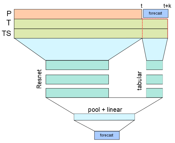
I built a model that takes as input the past (24 hours) plus the forecast of the Temperatures and predicts the Power P for the next 6 hours.
I treated the past 24 hours with a ConvNet and the forecast of the explicative variables with a Tabular model. Then I mixed the feature map of the ConvNet with the output of the tabular model appending a classic resnet head.
The output is pretty good, probably my architecture is kinda of noobish, so suggestions are welcome!

My Dataset is a Double input dataset, just to concatenate both different size arrays (TimeSeries):

class DoubleDataset(Dataset):
    def __init__(self, X, X2, y):
        self.X = X
        self.X2 = X2
        self.y = y
        
    def __len__(self):
        return self.X.size(0)
    
    def __getitem__(self, idx):
        return (self.X[idx], self.X2[idx]), self.y[idx], 

and my model:

def basic_conv():
    return   nn.Sequential(nn.Conv1d(3, 64, kernel_size=3, stride=2, padding=1),
                           ResLayer(64),
                           ResLayer(64),
                           ResLayer(64),
                           AdaptiveConcatPool1d(),
                           Flatten(),
                           )
def tabular_model(inc:int, out_sz:int):
    layers = [Flatten()]
    layers += [nn.Linear(inc, 1000)]
    layers += bn_drop_lin(1000, 500, p=0.01, actn=nn.ReLU(inplace=True))
    layers += bn_drop_lin(500, out_sz, p=0.001, actn=None)
    return nn.Sequential(*layers)


class mix_model(nn.Module):
    def __init__(self, inc:int, out:int):
        super().__init__()
        self.cnn = basic_conv()   
        self.tabular = tabular_model(inc, out)
        self.head = nn.Sequential(*bn_drop_lin(64*2+out,256, p=0.1, actn=nn.ReLU(inplace=True)),
                                  *bn_drop_lin(256, 256, p=0.01, actn=nn.ReLU(inplace=True)),
                                  nn.Linear(256,out)
                                 )
    def forward(self, x1, x2): 
        y = self.cnn(x1)
        y2 = self.tabular(x2)
        y3 = torch.cat([y,y2], dim=1)
        return self.head(y3)

[akshayb7 (Akshay Bhardwaj)]

Hi Marc, thank you for such a detailed and thorough reply. It is indeed intended to be monitored online. I will go through all the resources listed by you to understand and then apply them to some of the sample data available to me. The DWT one looks particularly helpful and should be fun to tinker around with. I’ll experiment on these methods throughout the week and will definitely share my results with you and everyone else. Cheers!

[marvin (Marvin Hansen)]

Has anyone experience with Data augmentation for Time Series Forcasting?

I did a quick internet search today and was kinda dumbfounded to learn that this field seems to be rather under construction. Has anyone any actual experience beyond window sliding?

Edit: Found a nice toolkit from a 2017 paper:

Data-Augmentation-For-Wearable-Sensor-Data

Github: https://github.com/terryum/Data-Augmentation-For-Wearable-Sensor-Data/blob/master/Example_DataAugmentation_TimeseriesData.ipynb

https://sites.google.com/site/machinelearningforfun/basics/data-augmentation-for-time-series

Data Augmentation strategies for Time Series Forecasting

[marcmuc (Marc P. Rostock)]

This looks interesting. The two “augmentation” methods I have seen used most in kaggle competitions are

• augmenting by adding gaussian noise
• dropping a percentage of the original measurements (kind of like input dropout)

And I just realized it might be an interesting method to randomly drop a certain percentage of timesteps and then close those gaps with potentially different forms of interpolation / missing data treatment. That way there should be changes that kind of stay consistent with the acutal series, but change it in small ways. Maybe combined with a little noise? Never tried that though…

The two recent competitions you might want to search the top 10 solutions for these kinds of things are the PLASTiCC and the VSB Power Lines ones, but there are older ones that also might have interesting stuff… Both were for classification, not forecasting though.

[tcapelle (Thomas)]

Does anyone have a Timeseries forecasting notebook using RNNs?
I am trying to reproduce the lesson 7 notebook (human-numbers) with Time series data but I am having a hard time.
https://machinelearningmastery.com/how-to-develop-lstm-models-for-time-series-forecasting/
I am trying to reproduce this trivial examples in pytorch/fastai and I am failing miserably…
Basically, make an RNN to predict a linear regression…
Any hints?

tcapelle/RNN_study/blob/master/Basic RNN.ipynb

[marvin (Marvin Hansen)]

@marcmuc

When reading the paper corresponding to the wearable data augmentation stuff, it struck me that the most effective methods were identical or very similar to what is used in image augmentation. Int he published benchmark, the authors were able to boost classification accuracy by up to 10%. I hope to test that out next week as to see how it works on my time series data.

Adding Gaussian noise is certainly a best practice worth measuring. I think input dropping is already done implicitly in fast.ai whenever you use regulation.

That said, I already have ~15 more experiments on my bucket list so I hope to get some results next week. In case something interesting pops up, I share an update.

[nok]

What a shame that he earns a lot star on github and medium’s attention by fooling others in this way…

[marcello_m (Marcello Morchio)]

Hi All!
i am very new here so sorry if I ask basic things. I am attempting to apply the image transformations to time series as showed by @oguiza back at the beginning og this thread. I had my hard times in realizing the the pyts libray is now in rev 0.80 and the GASF, GADF, MTF, RecurrencePlots classes have been renamed. Some have been suppressed.
OK, rolling back to 0.70 it is much better, but still I cannot run properly the MTF tranformation.
Executing the cell with

mtf = MTF(64)
X_mtf = mtf.fit_transform(X_train)

in the gist I get an error

~\AppData\Local\conda\conda\envs\pyts\lib\site-packages\pyts\image\image.py in _mtf(self, binned_ts, ts_size, image_size, n_bins, overlapping, window_size, remainder)
    334                 for j in range(image_size):
    335                     AMTF[i, j] = MTF[np.arange(start[i], end[i]),
--> 336                                      np.arange(start[j], end[j])].mean()
    337 
    338             return AMTF

IndexError: shape mismatch: indexing arrays could not be broadcast together with shapes (15,) (16,) 

Looks like there is some rounding somewhere in the library and one index which should be sqrt(64) becomes 15.
I can bring on my investigation skipping the MTF transformation, still this is pretty annoying!
Any hint?

[hwasiti (Haider Alwasiti)]

And what about multivariate time series?

There are several approaches you could follow.
In all cases you would first transform each individual TS within a MTS into an image (array).
Some alternatives are:

1. Tile images to build a larger image.
2. Stack all images into a multichannel (3+) array.
3. Fuse the images into a single image.
   To perform 2 & 3 you would need to modify the convnet to allow 3+ channels.

Thank you for the excellent post @oguiza
Here is an examples for (1):

1. This is something I am working one. Multiple EEG sensors on the scalp. So this is an example of multi-variate time series (each electrode position will pick up a signal that we are interested in its spectrograms, so we have 64 spectrograms). Have a look into the image with the black background :

I add to your list:
4. Concatenating multi CNN outputs (each CNN for each uni-variate spectrogram) into single dense NN like this:

How to remove the last fully connected layer from a CNN in fastai to stack more than one CNN into a FC-NN?

There are ML problems when we need to stack more than one model. Take for example chest X-Rays need stacking 2 CNNs for front and lateral views like this model : [ScreenClip] Source The above method is way better than stacking 2 full CNN into FC (which is I am aware it is doable with fastai) like this: [ScreenClip] Because the output of each CNN in the 1st image has way more features describing each xray image, which is crucially important… Since the physician will not be able to classify …

[oguiza (Ignacio Oguiza)]

Hi @marcello_m,
I’ve checked the updated pyts library and it seems to me that all the functionality to transform time series into images is still there. They’ve modified the API though, so you can still get access to all 4 image transformations I used in the gist. They actually have examples of how the new functionality works here. I don’t have time to update the gist right now, but I’m planning to create some notebooks to demonstrate the different alternatives in the next few weeks.
In any case, I’d recommend you update to the latest version and follow the examples to update your copy of the gist.
Please, let me know if you can make it work or find another issue.

[fuelnow (George Zhou)]

Hi everyone, really glad to have found this group. I am working on developing a model that can forecast (1 or more time steps) using varied time steps in the past (e.g. 64,128,256) and multivariate inputs using CNN. The results are rather good but I was looking into ways to make it better. Has anyone tried time series forecasting using the MTF,recurrence plots, or GAF (e.g. using the pyts library) and can share their experiences/results/wisdom? It seems that most reported results I have seen have been on using pyts for classification rather than forecasting.

[oguiza (Ignacio Oguiza)]

Wow, this is really interesting! Thanks for sharing @hwasiti!

Multiple EEG sensors on the scalp.

I’d have some comments/ questions on this:

• Are you using a public dataset or proprietary data?
• What level of performance (accuracy?) do you get with this approach?
• Have you compared this approach (time series to image transformation) to the more standard time series as array approach (using FCN, ResNet, etc)?
• Which of the images above do you use as input into the nn?

I add to your list:
4. Concatenating multi CNN outputs (each CNN for each uni-variate spectrogram) into single dense NN

Absolutely! I missed this approach which I think makes a lot of sense. I’ll add it to my previous response for completion and will create a link to your post. Thanks for adding this alternative!

[oguiza (Ignacio Oguiza)]

Hi @fuelnow,
I have not used the time series to image approach for forecasting, but think it should also work.
I don’t know if anybody else has tested it, but it’ll be great if you try it and share your experience!

[fuelnow (George Zhou)]

yeah, i can post some of my findings here! Has anyone received this error while using the pyts package (specifically MarkovTransitionField) before?
/usr/local/lib/python3.6/dist-packages/pyts/preprocessing/discretizer.py:148: UserWarning: Some quantiles are equal. The number of bins will be smaller for sample [ 0 2 6 9 10 14 17 18 22 30 31 35 42 44
50 52 54 56 58 59 61 63 66 70 78 79 80 82
85 89 97 99 100 101 102 107 109 111 113 114 115 119
125 128 132 135 141 143 147 152 154 161 164 166 170 183
193 195 197 198 211 213 220 225 228 230 234 242 247 251
252 259 260 261 263 264 275 277 284 285 287 300 305 310
313 326 328 329 330 331 332 333 337 340 348 349 351 352
353 358 361 363 364 374 377 378 379 387 390 393 401 405
406 407 408 409 410 413 414 419 423 424 426 428 433 439
442 446 447 449 450 455 456 461 463 465 469 475 478 483
490 491 492 495 500 505 506 511 514 515 522 532 534 535
544 547 548 550 553 564 566 567 569 574 577 579 583 585
590 594 596 597 598 602 603 610 611 613 615 616 618 619
620 626 629 633 644 645 646 648 650 651 652 659 661 665
667 668 670 676 679 681 684 688 690 691 695 716 718 719
721 725 739 740 744 750 753 754 757 760 763 765 770 771
777 778 780 784 790 791 794 800 805 808 809 810 813 818
838 846 854 855 860 863 871 872 874 884 886 889 893 896
903 906 909 911 917 922 928 929 930 932 938 940 946 951
953 954 955 957 961 962 965 966 972 975 976 978 981 983
984 988 992 999 1000 1002 1005 1009 1010 1011 1012 1014 1020 1028
1032 1036 1042 1043 1046 1047 1051 1060 1066 1073 1074 1075 1090 1098
1103 1106 1107 1108 1113 1114 1118 1121 1125 1134 1140 1141 1144 1145
1146 1152 1153 1154 1158 1160 1166 1167 1170 1171 1172 1173 1174 1179
1181 1187 1192 1198 1202 1207 1211 1212 1222 1223 1229 1233 1236 1247
1249 1251 1253 1259 1261 1265 1266 1273 1277 1281 1285 1287 1291 1293
1298 1299 1306 1313 1315 1316 1320 1333 1336 1338 1342 1345 1347 1351
1355 1358 1359 1362 1369 1371 1372 1376 1377 1378 1385 1386 1390 1393
1395 1398 1399 1400 1401 1404 1405 1409 1415 1418 1423 1424 1425 1429
1434 1437 1438 1444 1456 1458 1462 1464 1466 1467 1471 1473 1476 1481
1485 1486 1487 1495 1497]. Consider decreasing the number of bins or removing these samples.
“of bins or removing these samples.”.format(samples))

[oguiza (Ignacio Oguiza)]

Yes, I’ve experienced something similar in the past.
Here’s how MTF works:

Markov Transition Field (MTF): the outline of the algorithm is to first quantize a time series using SAX, then to compute the Markov transition matrix (the quantized time series is seen as a Markov chain) and finally to compute the Markov transition field from the transition matrix.

So a key step is to split the y axis of the time series in bins. N_bins is a hyper parameter you need to specify. Some restrictions to the number of bins you can use: greater than 2 and less or equal to the number of timestamps. You can experiment with it. Something I’ve used in the past is timesteps//2, timesteps//4, etc. As a result, you will see that the resulting image has more or less granularity.