Retina Net

I have tried to reproduce a RetinaNet in this notebook with a resnet-34 backbone and trained it for a bit. Not sure it’s properly done since the mAP dropped from 30% to 20% (computed with the same method we used with @daveluo).

I’ll try to take a look into the details to see what’s going wrong, and I also completely skipped the way they compute the predicted boxes to use the same as in the pascal notebook. I’ll dig into that later, I wanted to focus on the architecture first.

In the meantime, any feedback is welcome!

12 Likes

I believe @groverpr and @kcturgutlu are looking at this too so cc’ing them

2 Likes

@shik1470 also :slight_smile:

@sgugger Thanks for sharing the notebook. We started it yesterday. Give sometime before any fruitful discussion/ feedback.

I implemented the anchors like they did it in the paper (or so I think) but somehow made it worse… 17.6% of mAP now. Not sure what’s wrong with the code though, because the anchor encoding/decoding seem to work properly.
Anyway, it’s in this notebook if you have time to check.

2 Likes

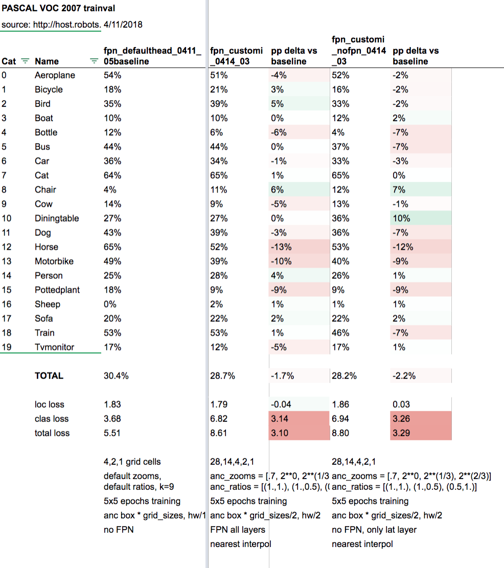
I’ve been trying to implement a FPN as well and running into similar issues where everything I’ve tried performed worse than my baseline: a nearly default pascal-multi that gives mAP=30.4%. Here’s my baseline notebook.

The best mAP with my FPN implementation I got so far is 28.7% using a [28, 14, 4, 2, 1] scale pyramid with k=12. Thanks @sgugger for some helpful functions and techniques in customizing the model. Here’s that notebook: https://github.com/daveluo/fpn/blob/master/FPN_heavycustom_0414.ipynb

I’m not faithfully recreating retinanet in full - just applying the concept of a FPN (correctly I hope) to the default pascal-multi resnet34 backbone and head to try to improve its performance.

I’ve tried systematic variations using every scale level from 56 to 1, a range of zooms and aspect ratios, different matching and NMS thresholds, bilinear vs nearest interpolation for upsampling, etc. but they all performed worse.

To see if my FPN implementation did anything at all, I removed the lateral+upsamp step from my best implementation and directly connected the lateral kernel_size=1 conv outputs to my outconvs at each scale level. Keeping everything else the same, this gave a mAP of 28.2% so there seems to be a small (+0.5% mAP) benefit to the upsampling and addition step. Maybe that’s an insignificant difference? Here’s that notebook: https://github.com/daveluo/fpn/blob/master/FPN_heavycustom_0414-nofpn.ipynb

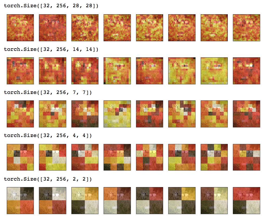
To debug and better understand what’s happening, I used pdb and stepped through the forward loop to confirm each part happened as expected. I also used the heatmap technique to visualize outputs at each scale. Looks like what we should expect:

Compare this to the notebook where I skip the lateral+upsamp step (note the difference of activation near the cows at each scale):

So I’m also still at a loss for where our implementations are going wrong :confused: I don’t think the mAP calculation is wrong because I’ve found that my visual inspection of the predictions vs gt bboxes lines up pretty closely with changes in the mAP and it is calculating as I’d expect in other applications.

Also if helpful, here’s a comparison of the class APs and loss scores across the 3 models I’ve referenced and linked (baseline vs FPN vs not-FPN):

6 Likes

A bug that I had in the first version of my code is that I wasn’t flattening the conv outputs in the correct order, so the receptive fields didn’t match to the anchor boxes. Have a look at conv_flatten in my notebook to see how I (think I) fixed this.

Hmm, I was just about to ask about this because my model isn’t learning anything plus I am starting with a loss around 10e6, which I couldn’t find a reason for. @daveluo very cool visualizations and also thanks to @sgugger ! You guys are way ahead of me I hope I can debug my code and get some results to compare with yours.

What I am trying:

  • Using initializations for both weights and biases mentioned in the paper. Which is gaussian (0, 0.01) for weights bias =0. Except for output layer of classification subnet which has bias = np.log((1-pi)/pi) with pi = 0.01
  • Same aspect ratios and zooms for anchor boxes total 9.
  • Pascal Dataset.
  • sz = 256 and FPN levels of 4x4, 8x8, 16x16, 32x32, 64x64.

Here is the notebook: https://github.com/KeremTurgutlu/deeplearning/blob/master/pascal-retinanet.ipynb

Yes, I’m using your latest version of flatten_conv but checking that the network spitting the anchors in the correct order is next in my things to check in debug.

That’s why I started with just 4 anchor boxes - i.e one layer of outputs with a 2x2 grid and just 1x1 aspect ratio. Easier to debug and visualize. It’s nearly impossible to debug if you can’t visualize it and step through a debugger printing the outputs.

1 Like

UPDATE 4/17: the below fix and discussion is specific to our own notebooks posted above in this thread. The official pascal_multi notebook has the correct implementation and does not need to be changed. I will be updating my notebooks going forward to sync up with the official version. Sorry for any confusion.


Found the issue! (…well, at least one issue :))

@jeremy, your suspicion was correct - our flatten_conv function was not correctly lining up the order of anchor/prediction bboxes with that of the receptive fields.

Anchor/prediction boxes were incrementing by going top–>down each column first and then the next-right column while the receptive fields were going left–> right first and then down to the next row.

The fix is to switch the permute dim-ordering (x.permute(0,3,2,1) instead of x.permute(0,2,3,1) so that we are transposing the order of our prediction boxes as we flatten our outbound convolutions:

def flatten_conv(x,k):
    bs,nf,gx,gy = x.size()
    x = x.permute(0,3,2,1).contiguous()
    return x.view(bs,-1,nf//k) 

Running my baseline pascal-multi notebook, this improved mAP from 30.4% to 32.4%

In my best performing FPN variant so far, the fix improved mAP from 31% to 35.7%! Notebook link coming soon…

On visual inspection, the effect of the bug is obvious (but only in retrospect…). I was seeing a lot of weird localization errors like this:

After the fix:

No more sheep in the trees!

This bug has the greatest effect where gt objects are clustered to the bottom left or top right and our prediction boxes are transposed to the other side of the diagonal. The prediction bboxes still tried to make their way towards maximum IoU with ground truth but there was only so far they could go due to the center and height/weight constraints we set.

It wasn’t that obvious by just comparing the average localization and classification loss values:

Pre-fix:
loc: 1.8269546031951904, clas: 3.6849770545959473
5.5119

Post-fix:
loc: 1.8288934230804443, clas: 3.7000365257263184
5.5289

Now we’re in business! I’m sure there are still issues/tweaks to be made on the FPN side of things so I’m looking forward to seeing how high we can push the mAP.

13 Likes

Very good catch! On Jeremy’s notebook, a quick run made me go from our 30% mAP benchmark to 31.8% so it’s clearly better.
I’ll try to see what it gives me on the Retina notebook!

So the bug is also in my notebook? :open_mouth: I better fix it…

1 Like

Yes, because we all copied you :sweat_smile:

4 Likes

Well you won’t make that mistake again…

1 Like

Good news: my best mAP is now at 37.4%.

Bad news: my FPN implementation made things worse (dropped mAP to 35.7%). I compared models by directly connecting my “c” feature maps at each level to outconvs (skipping lateral, upsamp, addition, smoothing steps in FPN).

Looks like the addition of many more anchor boxes (12,012 to be exact) at smaller scales (28x28, 14x14) plus the fix to flatten_conv helps detection performance. But my FPN is not working yet.

Here are the key settings that I changed from default:

anc_grids = [28,14,4,2,1]
anc_zooms =  [.7, 2**0, 2**(1/3), 2**(2/3)]
anc_ratios = [(1.,1.), (.5,1.), (1.,.5)]
len(anchors), k
  (12012, 12)
pi = 0.01; bias = -np.log((1-pi)/pi)

And here’s the notebook: https://github.com/daveluo/fpn/blob/master/fpn_customk_nofpn_0416_05_flattenconvfixed-public.ipynb

3 Likes

Well I’m confused… My loss on pascal-multi is much worse with this change, and the predictions are visibly much worse too. Have you got the latest version of the notebook from github? And if you use that with no other changes but the permute in flatten_conv it gets better?

My apologies, it’s my version of your notebook that we then used with @daveluo to compute the mAP that has the bug, the pascal-multi notebook has the anchors centers going up by lines then columns (and we have that transposed).
No need to do this in the notebook in short.

2 Likes

Whoops sorry about the confusion - I didn’t realize either that the manner in which anchors are created changed between our notebook and the official one. Will be more careful going forward to check the diff.

Update: To pinpoint and clarify exactly how we went off-track…

Our version:

anc_x = np.concatenate([np.tile(np.linspace(ao, 1-ao, ag), ag)
                        for ao,ag in zip(anc_offsets,anc_grids)])
anc_y = np.concatenate([np.repeat(np.linspace(ao, 1-ao, ag), ag)
                        for ao,ag in zip(anc_offsets,anc_grids)])

for anc_grids=2 and k=1, produces anchor_cnr:

Variable containing:
 0.0000  0.0000  0.5000  0.5000
 0.5000  0.0000  1.0000  0.5000
 0.0000  0.5000  0.5000  1.0000
 0.5000  0.5000  1.0000  1.0000
[torch.cuda.FloatTensor of size 4x4 (GPU 0)]

which draws the anchor boxes going top–>down each column (note the number of each box: 0, 1, 2, 3)
image

Official pascal-multi version:

anc_x = np.concatenate([np.repeat(np.linspace(ao, 1-ao, ag), ag)
                        for ao,ag in zip(anc_offsets,anc_grids)])
anc_y = np.concatenate([np.tile(np.linspace(ao, 1-ao, ag), ag)
                        for ao,ag in zip(anc_offsets,anc_grids)])

produces anchor_cnr:

Variable containing:
 0.0000  0.0000  0.5000  0.5000
 0.0000  0.5000  0.5000  1.0000
 0.5000  0.0000  1.0000  0.5000
 0.5000  0.5000  1.0000  1.0000
[torch.cuda.FloatTensor of size 4x4 (GPU 0)]

which draws the boxes going left–>right and then next row down:
image
This is the correct arrangement of boxes that lines up with how the receptive fields are ordered (left–>right and then next row)

The only difference between the two versions is the order in which we use np.repeat and np.tile for anc_x and anc_y. Given [0,1] and repeats=2:

  • np.repeat makes [0,0,1,1]
  • np.tile makes [0,1,0,1]

So switching the order of the functions as applied to anc_x and anc_y flips the x,y coordinates (0,1) <–> (1,0) and transposes the ordering of the anchor boxes.

Subtle yet important difference! as I’ve unwittingly discovered…

2 Likes

After visually looking at slices from the tensor, this is how flatten_conv works in my opinion:

def flatten_conv(x, A):
    """
    IMPORTANT: Receptive fields should match : target-output
    A: number of anchors
    
    Flatten output as row by row:
    grid row 0 col 0 anchor 0
    grid row 0 col 0 anchor 1
    ...
    grid row 0 col 1 anchor 0
    grid row 0 col 1 anchor 1
    ...
    grid row 0 col 2 anchor 0
    grid row 0 col 2 anchor 1
    ...
    grid row n col n anchor A-1
    grid row n col n anchor A
    """
    bs,nf,gx,gy = x.size()
    x = x.permute(0,2,3,1).contiguous()
    return x.view(bs,-1,nf//A)

Anchor creation also seems to be consistent sliding row by row for each pyramid level:

2 Likes

It’s so nice you got it working! I didn’t get the time to go back on it last week but I’d like to see if I can get comparable results with their way of interpolating the bbox; I see you’ve just clamped the outputs of the network.

Dividing the class loss by the number of matched anchors helped for me as well (it was a recommendation in their paper), I’ll try the other tweaks.