You definitely need to do lr_find before you train, otherwise there’s no point running lr_find!.. I suspect I’m not really understanding your question…
No you don’t have to create a new learner. The LRs are a param to fit(). You can also pass them as a param to lr_find(). Now I think about it, we didn’t actually cover this on Monday! I’ll mention it in the next class. Basically, do something like this:
If you’re feeling generous, a pull request with docs for those params would be nice! Especially to point out that you can pass differential learning rates to lr_find, and it’ll keep the multiples between the groups constant (but the plot will show the LR in the last layer group). No obligation though - only if you feel like it!
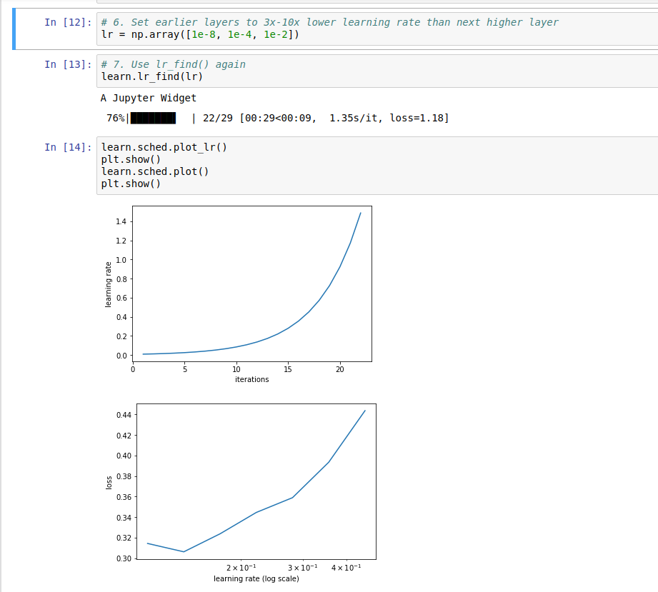
… but when I tried to plot it via learn.sched.plot(), the plot looks way off (I can’t screenshot it, but it’s a diagonal line going up from left to right).
lr = 1e-2
... train
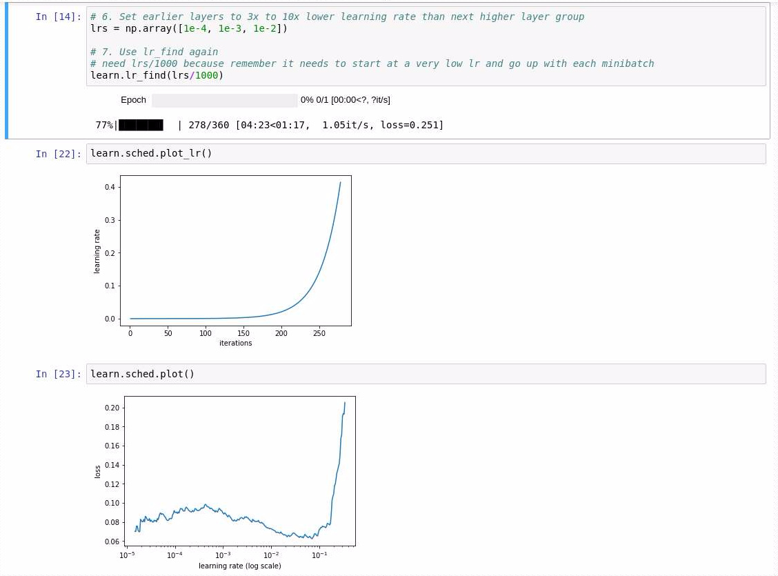
lrs = [1e-4, 1e-3, 1e-2]
learn.lr_find(lrs/1000)
# looking at learn.sched.plot() the most optimal learning rate is 1e-5,
# so before more training I update my "lrs" variable accordingly ...
lrs = [1e-7, 1e-6, 1e-5]
learn.fit(lrs, 3, cycle_len=1, cycle_mult=2)
Is that a correct understanding of using and applying what we learn from lr_find()?
Right. But given that this is Step 7 (of 8) in “easy steps to train a world-class image classifier”, the network would naturally already be pretty trained. Indeed, prior to this I’ve trained the last layers both with and without data augmentation by the time I run this.
If this is indeed the expected graph, how would you interpret the second plot? Would the appropriate learning rate for the last layers of the network be maybe somewhere between 10-3 and 10-2?