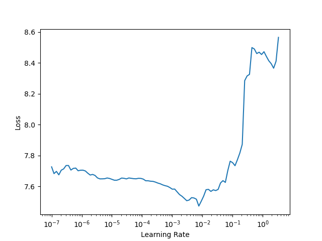
so in the first graph (before fine tuning the model) you see the loss is high(7.7) for the lower learning rates and as you increase lr the loss drops until your lr is too large and it starts to diverge.
Now once your model is trained your weights have moved closer to the “desired weights” so your loss should be lower and you’ll need to take smaller steps from now own so that you don’t oscillate/diverge.
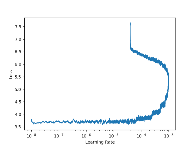
When you run lr_find now you see a lower loss (3.7) since the weights are closer to the “desired weights”.
So based on the first graph you probably used say 10e-3 to train but in the second graph you see 10e-3 is way too large a step size.
Kind of hand wavy hope you get the intution.
Little bit of history:
Before fine_tune existed you had to:
freeze all layers but the last,
run lr_find, choose a lr,
train,
then unfreeze all layer and choose multiple lrs to train different sections of the layers,
run lr_find,
choose multiple lrs and train again.
Now all this is automatically done in fine_tune. A peak into that source code should help too.
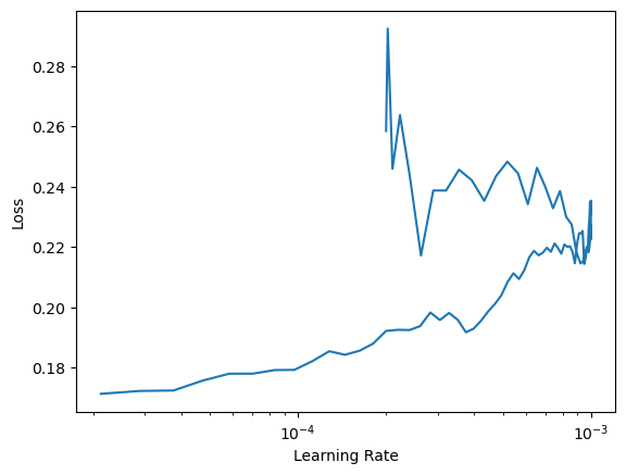
I was actually wondering how it is possible to get a curve where x-values can have multiple y-values. For example, for each learning rate between 10e-4 and 10e-3, there are two loss values.
So based on the first graph you probably used say 10e-3 to train but in the second graph you see 10e-3 is way too large a step size.
Does this mean that I should not trust the training output? When I apply the resulting model on a few samples, the inferences are rather correct.
Now all this is automatically done in fine_tune.
Thanks for the info! I did not know that fine_tune contained all these steps. I was currently using fit_one_cycle.
think of a parabola where you know the minimum loss is at the bottom, before training the model you are at the upper end of the parabola. Your goal is to get the minimum loss which as at the bottom. Now you can take large step to reach the bottom but once you are at the bottom you need to reduce those step sizes or else you’ll oscillate.
Now similarly the first lr_plot shows you a much higher loss since you are further away from the “ideal weights”. to get the “ideal weights” you take larger steps. Now your loss is reduced, your model is doing a reasonable job. Now you plot the lr_plot again your loss is lower(makes sense as you trained your model partially) the lr in the plot is smaller (like you are at the bottom of the parabola).
like you see the inferences are correct, the two different lrs are because you are at two different stages of training. Stage one you use a higher lr as you are further from your optimum. Stage two you use a lower lr as you are closer to your optimum.
In which context are you calling plot_lr_find? I think it is not designed to call it manually but rather use learn.lr_find. The only thing that plot_lr_find does is checking the learners recorder (thats the thingy that keeps track of all kinds of parameters during training) and plots the recorded learning rate against the recorded loss.
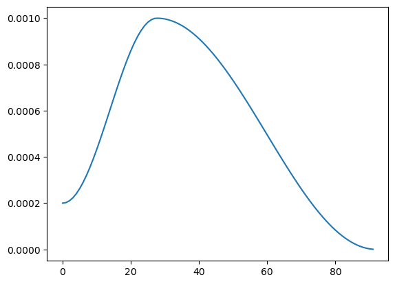
A (default) learner uses something called cyclic learning rates, meaning (as @barnacl already hinted) the learning goes up and down during training, which looks like this:
As you can see: most learning rates are getting used twice, thats why you see two x-values when calling:
learn.recorder.plot_lr_find()
Note that in this figure, values lower than ~2e-4==0.0002 have only one x-value, this corresponds exactly to the ‘tail’ of the learning rate plot in the first figure, which is only used once during training.
That roughly resembles what I expected in my explanation above (second plot_lr_find is called after training and thus plots the values captured during training, where the lr goes up and back down). Is this enough then or do you need something clarified?
Also, in my humble opinion, you don’t need either of the two:
blocks, especially if you copied that code and don’t have a particular reason to run them. (Again: in my opinion) the lr_find plot isn’t a usefull artifact to save, what could make sense to save is how the loss behaves at each epoch during training which is saved in learner.recorder.losses.