Part 1, online study group

[msivanes (Manikandan Sivanesan)]

Meeting Minutes 16-02-2020

Topic: Lesson 5, Part 1

Start Time: Feb 16, 2020

Recording

Presenter: @gagan (Huge thanks for an excellent learning experience)

Disclaimer: Any mistakes in the notes are solely mine and not of the presenter. If you find any mistakes, please provide feedback in the comments so that I can correct them.

Agenda

• Deep Learning internals with backpropagation
• Fine-tuning in Transfer Learning
• Learning Rate tricks: Annealing, Discriminative LR
• Weight Decay
• Momentum + RMSProp => ADAM
• Mnist SGD with Cross-entropy and softmax

Meeting Notes

• Deep Learning internals with backpropagation
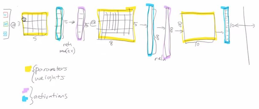
  • Weights & Biases are the parameters that are typically learned.
  • the output of the matrix multiplication or result of calculating something are called activations
    
    
  • Affine functions : linear functions (a + b ) * c -> this will result in another affine function (another linear).
  • Why non-linearity? Real-world is not linear, hence we definitely need to introduce non-linearity. In order to model the real world, that’s why ReLU s are needed.
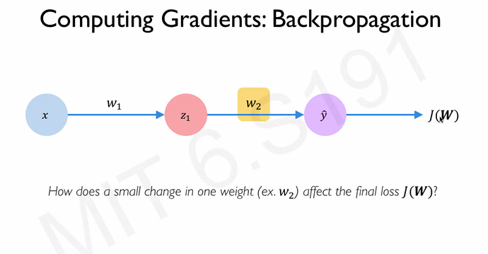
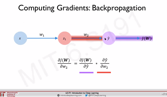
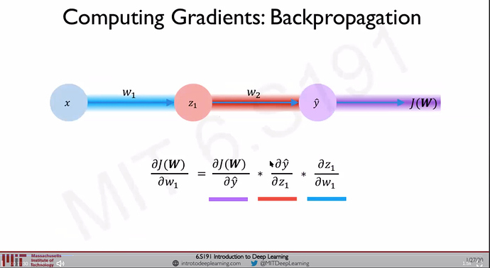
  • Backpropagation: Chain rule: How does a small change in one weight (eg: w2) affect the final loss J(W) Source: [1]

• Bias/Variance tradeoff [2]

  • High bias(underfit)
  • High variance (overfit)

• More number of parameters does not necessarily mean Higher Variance. Deep Learning can have more number of parameters but use Regularization to penalize for complexity.

• Fine-tuning in Transfer Learning

  • why freeze? What happens when we freeze?
    • It replaces that last layer with newly added two layers (layer groups) with ReLU in between.
    • Earlier layer weights are good at identifying shapes, color, etc & hence frozen. Only the last layer weights (initially random) are set up for learning that is task-specific (eg: classify pets)
  • why unfreeze & train the entire model?
    • Earlier layer weights are completely trained on a different dataset (eg: ImageNet, Wiki). They contain useful information but also contain not useful information for this specific dataset (eg: classify pets).

• Learning Rate tricks : Annealing, Discriminative LR

  • Leslie Smith paper
  • plots loss vs learning rate
    • 1e-3 -> all layers same lr
    • slice(1e-3) : (final layers=1e-3, rest = (1e-3)/3) . Lower learning rate for the earlier layers because they are near to an optimum label & to avoid overshooting.
    • slice(1e-5, 1e-3). 1e-5 applied to first layer group, 1e-3 to last layer group and somewhere in between for middle layers
  • Applying different learning rate to different layer groups is called Discriminative Learning Rates.
  • 3 layers groups are the default for CNN

• Gradient Descent

  • What is the difference between vanilla Batch GD (avoiding confusion by adding vanilla) , SGD, Mini Batch GD?. We use MiniBatch GD. For more information see this post [5]
  • Too much of batch size lead to Out of memory error (meaning batch size is too high)
  • SGD is used during Online learning (product environment) - learning (training) on the go - batch_size is typically 1

• MNIST - SGD
  See this post for code & explanation

  • Neural Network without hidden layers => Logistic Regression

  • Notebook walkthrough lesson5-sgd-mnist notebook

  • Mnist SGD with Cross-Entropy and Softmax (entropy_example.xlsx)

    • Softmax (& exponential) : finite, positive range, % of cattiness (the given feature) in this image. It guarantees
      • All the activations add up to 1
      • All of the activations are > 0
      • All of the activations are < 1
    • entropy : measure of chaos (lack of orderliness)
      • type of loss function
      • High Penalization for wrong answer.
      • Very low penalization for correct answer
    • Loss & Cost are almost similar & related.
    • Loss function (error for each sample) - difference between prediction & actual
    • Cost function (entire dataset or mini-batch) - average of the losses for the mini batch - hence loss function is part of cost function.
    • (Classification/ categorical : +cross-entropy. Regression/Continuous : RMSE)

  • Weight Decay : Makes the weight not overly significant

    • Weight Decay: (Source: Metacademy) When training neural networks, it is common to use “weight decay,” where after each update, the weights are multiplied by a factor slightly less than 1. This prevents the weights from growing too large, and can be seen as gradient descent on a quadratic regularization term.

    • Epoch vs Iteration

      • Let us consider a training dataset with 50,000 instances. An epoch is one run of the training algorithm across the entire training set. If we set a batch size of 100, we get 500 batches in 1 epoch or 500 iterations. The iteration count is accumulated over epochs, so that in epoch 2, we get iterations 501 to 1000 for the same batch of 500, and so one. [7]

• Learning Rate Annealing reduce the lr dramatically as we are nearing convergence.

• Polynomial functions can model anything. We can introduce a lot of complexity using a lot of parameters. Use Regularization to penalize complexity but still use a lot of parameters. One common way to do regularization is to use weight decay

• Momentum + RMSProp => ADAM

• a pure Pytorch setup for FashionMnist dataset.

Questions

See the above post

Advice / Action Items

• Watch at least the lectures 1 & 2 of Intro to Deep Learning from MIT [1]
• Go back and write backpropagation code in pure python [3].
• Too much of batch size lead to Out of memory error (meaning batch size is too high)

Resources

• [1] Youtube - Intro to deep learning
• [2] Bias/Variance TradeOff
• [3] Andrew Trask (@iamtrask) does the backpropagation in pure python Source
• [4] Building a minimal Neural Network from scratch
• [5] [Book] Grokking Deep Learning book by Andrew Trask for information about variants of Gradient Descents
• [6] Batch, Mini Batch & Stochastic Gradient Descent
  [7] The Cyclical Learning Rate technique
  [8] Softmax and Cross entropy loss
  [9] Link An overview of gradient descent optimization algorithms by Sebastian Ruder
  [10] Cost function vs Loss function

Misc

• Difference between Loss & Cost : The loss function (or error) is for a single training example, while the cost function is over the entire training set (or mini-batch for mini-batch gradient descent).
• Andrew Ng: ““Finally, the loss function was defined with respect to a single training example. It measures how well you’re doing on a single training example. I’m now going to define something called the cost function, which measures how well you’re doing an entire training set. So the cost function J which is applied to your parameters W and B is going to be the average with one of the m of the sum of the loss function applied to each of the training examples and turn.””
• Google says: The loss function computes the error for a single training example, while the cost function is the average of the loss functions of the entire training set