Hi all,
I am writing this as I went through the materials in course.fast.ai. Though I was not a formally registered student of course.fast.ai MOOC, I found the method of teaching deep learning by Jeremy Howard & Rachel Thomas is very interesting (and they are sharing this on the Internet for the world to learn), especially for me who does not have specific background in mathematics and just started to learn about deep learning.
I found this course somehow when I read a post by Yann LeCun of Facebook, a few weeks ago.
Sometimes, I tried to put things that I learn to a kind of article, then share to others in a few occasions. It aligns with my current job at the moment, in which one of the scope is to share to others on emerging technologies in computer science.
So here is my article as I completed the Part-1 of the course.fast.ai lesson-0 and lesson-1. Hopefully this can help others to start experiencing this excellent course, in the dynamic field of deep learning.
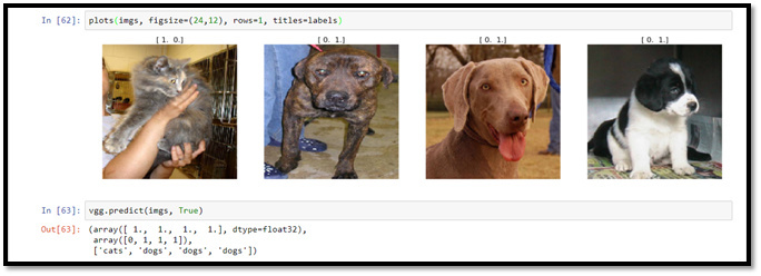
Illustration-1: Four images are recognized as cats or dogs based on pre-trained model in deep learning.
Human can naturally sense the things around them through many biological sensors like eye for vision, ear for hearing, nose for smelling, as well as skin for sensing heat and cold for example. That capabilities are just like embedded within us so we are just using those mostly unconsciously. They are all just there for us to use.
Machines on the other hand, can not be just be designed to have all those similar things like any normal humans can do. Years of research have been devoted to this, and many new advanced developments have emerged within just the last few years.
The invention of new algorithms, new optimization methods, new hardware are accelerating in this area of study with many potential practical applications. Illustration-1 shows the output of prediction of 4 images using certain algorithms. Those input images are recognized as dogs or cats, based on previously trained-model in deep learning, with 97.81% and 98.00% accuracy for Training & Validation data set, respectively.
The notable breakthrough of advancement in the field of computer vision using deep learning was in 2012 when an algorithm called Convolutional Neural Network (a.k.a. CNN) won the ImageNet competition “Image Classification challenge” by achieving error rate of 16.4%, significantly improved from 2011’s result which was at 25.8% (Fei Fei Li, Justin Johnson & Serena Young, CS231n lecture on Computer Vision @Stanford University in April 2017).
It was also mentioned that the subsequent results in 2013, 2014 and 2015 were at 11.7%, 6.7%, and 3.57% respectively. The 2015 ImageNet’s result has surpassed human expert (Stanford’s Ph.D student) that could achieve it at 5.1%.
Machine Learning & Deep Learning
Machine Learning is a subset of Artificial Intelligence (AI). Wikipedia defines AI as “Intelligence exhibited by machines, rather than humans or other animals.” One of sub-branches of Machine learning is Artificial Neural Network (ANN), which is a “mathematical model” of human biological brain. The simplest ANN (or just Neural Network) has 1 input layer, 1-hidden layer and 1 output layer as shown in Illustration-2.
Illustration-3 shows Machine Learning & Deep Learning within Artificial Intelligence framework.
Deep Learning is the current name of ANN in which it involves learning by utilizing more than 1-hidden layer (16 layers in VGG16, and 50 layers in RESNET-50 for example). Initially, machine learning can be categorized as Supervised Learning (labelled data) and Unsupervised Learning (non-labelled data). Recently, the 3rd category emerges: Reinforcement Learning.
Those 3 categories of Machine Learning are quickly summarized in table-1.
Machine learning offers the ability to extract certain knowledge and patterns from a series of observations. It’s all done through mathematical optimization by using models (pattern recognition or exploration of many possibilities). In supervised learning, minimizing the errors (as feedbacks) is very important to get the best learning result possible.
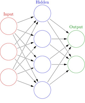
Illustration-2: A typical Artificial Neural Network (ANN) with 1-hidden layer.
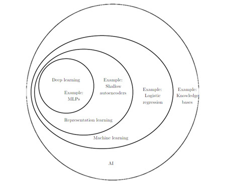
Illustration-3: Deep Learning within the Artificial Intelligence framework (source: MIT Press, deeplearningbook.org)
Deep Learning is all about Neural Network. It uses a lot of data to teach the machine to do things what human can do, see things and be able to recognize objects for example.
A friend of mine, Dr. Arfika Nurhudatiana, a data scientist in Jakarta, Indonesia recently emphasizes on this “Deep learning extends machine learning by excluding manual feature extraction and directly learns from raw input data.”
One of the good examples of Deep Learning application is perception. the ability for machine to be able to mimic human in recognizing images, see what objects are in the images, teaching the robot to understand the world around it and interact with it. Deep learning is the state of the art and emerging technology in Artificial Intelligence. Many applications are possible, including Computer Vision and Text/Speech Recognition with high degree of accuracy for example.
Each of the node in the hidden layer basically consists of complex calculations (mainly progressively matrix operations). It takes inputs from previous nodes – adjusted with unique biases (from nodes) and weights (from edges), then do some calculations (and measurements) to produce output to solve a problem. In Deep Learning, the hidden layers are more than one.
There are 9-hidden layers in Facebook’s DeepFace Neural Network. MIT Technology Review site reported in March 17, 2014 that Facebook’s DeepFace can have accuracy as high as 97.25%. While in average, a normal human being can do face recognition when presenting two photographs at 97.53% accuracy.
In VGG16 deep learning model, there are 16-hidden layers. VGG is the University of Oxford’s Visual Geometry Group that won 2014 ImageNet competition with 80% accuracy and considered state-of-the-art at that time (VGG-16 is the deep learning model that we will explore in this article along with the advances of processing approach with GPU in 2016-2017 – a recent lecture by Jeremy Howard, San Francisco University). The improved model can reach accuracy more than 97%.

Table-1: Three categories of Machine Learning.
**
Classification of Dogs & Cats, a Supervised Learning
**
PREPARING THE ENVIRONMENT
There is a recent deep learning class (2016-2017) taught in Silicon Valley in University of San Francisco by Jeremy Howard, a Kaggle’s #1 competitor for 2 years in a row and founder of course.fast.ai. Kaggle is a recognized place for competing for the best in the world in the area of deep learning by continuing to improve and invent the better algorithms (with million dollars reward for selected world-class’s tough challenges).
The class suggests to utilize GPU (Graphic Processing Unit) to run our deep learning training and testing (validation) and with this approach, we are using the one (virtual server) that is available in the cloud (with per hour-based charging). The configuration for NVIDIA GPU is shown in illustration-4 (idle) and illustration-5 (processing neural network).
As we can see, it is using the ubuntu distribution of linux operating system as the server for us to experiment, equipped with one NVIDIA GPU Tesla K80.
Once everything is setup, we can then start to use Jupyter Notebook to enter our python code to experience deep learning (python programming language is popular among data scientists). Note that we can opt to use our existing CPU-based laptop (Central Processing Unit) or CPU-based server without GPU, it’s perfectly fine.
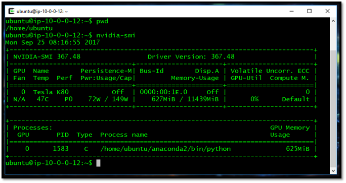
Illustration-4: State of single NVIDIA GPU: Tesla K80, with no process running – GPU Utilization is at 0%. The temperature is measured at 47oC, power consumption at 72W of 149W max, and GPU RAM usage at 625MB.
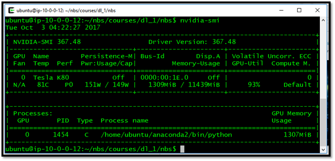
Illustration-5: State of single NVIDIA GPU: Tesla K80, when running neural network computations – GPU Utilization is at 93%. The temperature is measured at 81oC, power consumption at 151W of 149W max, and GPU RAM usage at 1307MB.
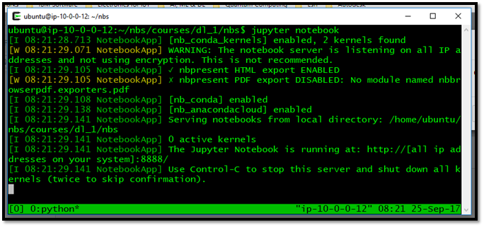
Illustration-6: A server equipped with one NVIDIA GPU, is running Jupyter notebook process which can be accessed from externally defined IP at port 8888.
However, the process will take significantly slow (About 10-20 times slower or more). The Neural Network processing that can take just a few minutes on GPU, can take hours if using CPU. This is the power of parallel processing embedded in GPU for processing complex parallel computations in Neural Network that are mostly consisting of matrix operations (linear algebra) & partial differentials formulas (calculus).
STARTING TO EXPERIENCE DEEP LEARNING
Ilustration-7 shows the python code within Jupyter Notebook, in which we are preparing the data & libraries to be used for training & recognizing images.
As a best practice as a data scientist, we usually do experimentation using set of small data, then apply the larger set of data once we have satisfied with the code that we develop (the training and validation process with a larger set of data requires certain amount of time, meaning the more we use GPU hardware, the higher the cost of processing those data set). This will reduce time in doing the extensive processing in GPU, and will be reducing cost per hour also if we are using cloud-based virtual server with GPU.
The preparation includes setting the path for data source (for training and validation), loading necessary libraries as well as initiating / instantiating variables to be used.
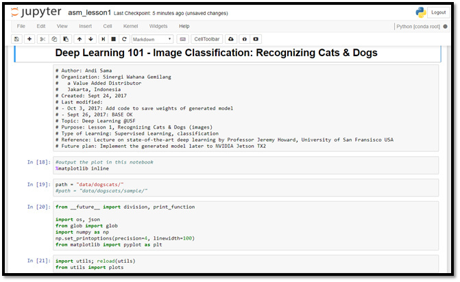
Illustration-7: Series of Phyton code that is preparing the execution of Neural Network. Major libraries being used are matplotlib for plotting the images, numpy for matrix computation and related utilities in utils.
THE 7-LINES OF CODE
1st step
Set the batch_size for data set (input), the number of input (images in this case) that are processed in parallel. 4 is the suggested number to start and experiment (based on experiment in October 2017, this consume about 1.3GB of memory in NVIDIA Tesla K80), unless we have a lot of GPUs and memories installed. For GPU memory as high as 12GB for example, 64 is the suggested maximum for batch_size.
2nd step
Import Vgg16 class (pre-trained deep learning model from ImageNet).
3rd step
Instantiate Vgg16 object to be used in the python code.
4th step
Prepare data set (images) for training using Vgg16’s instantiated object from a previously defined path (directory), number of images to be processed at a time according to defined batch_size.
5th step
Prepare images data set for validation using Vgg16’s instantiated object from a previously defined path (directory), number of images to be processed at a time according to defined batch_size.
6th step
Set instantiated Vgg16 object to finetune (prepare to retrain model using new data set). With the expectation that the accuracy will be better than before.
7th step
Execute the training and validation using pre-trained vgg-16 deep learning model, with new defined data set, and with certain number of epochs.
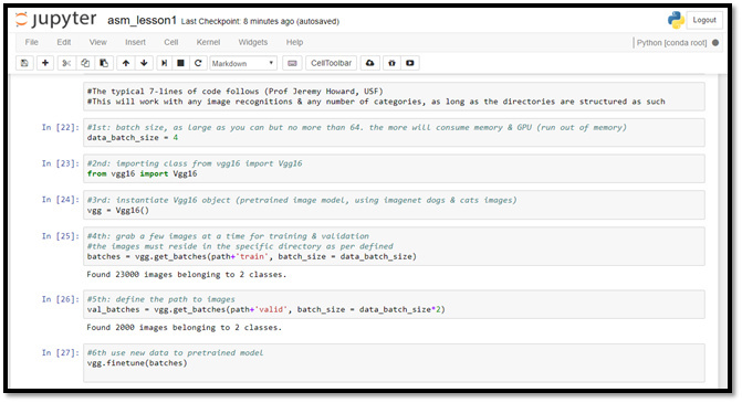
Illustration-8: The first 6-lines of 7-lines code to train images (credit: Professor Jeremy Howard , University of San Francisco).
EPOCH
One time iteration of training & validation with a set of data set is called 1 epoch. The training and validation can be repeated several times to improve the accuracy, although at some point the accuracy may be decreased. It is suggested then, to save the generated file (model) for each epoch (contain learned weights for all connected layers in the model).
Illustration-9 shows : 1st snapshot illustrates that the 1st epoch has been completed and the 2nd on start running (on Oct 3, 2017 GMT+7). As measured (2nd snapshot), it took 11’36.39” to complete the 2nd epoch on 1 GPU Tesla K80 configuration. This process completes 3 epochs with final accuracy on training data set: 97.81% and on validation data set: 98.00%.
As long as we have a source code (e.g. Vgg-16 in this example) and the generated weights file, we can duplicate to generate the same deep learning model in the future.
See illustration-10 on a generated file after 3 epochs. The file size is about 530+ MB.
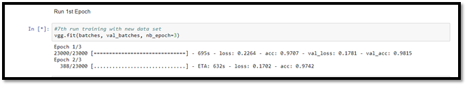
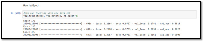
Illustration-9: 1st snapshot illustrates that the 1st epoch has been completed and the 2nd on start running (on Oct 3, 2017 GMT+7). As measured (2nd snapshot), it took 11’36.39” to complete the 2nd epoch on 1 GPU Tesla K80 configuration. This process completes 3 epochs with final accuracy on training data set: 97.81 & on validation data set: 98.00%.
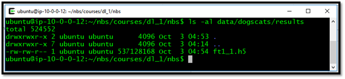
Illustration-10: The result file (model with all the weights) about 530MB after the 3rd epoch.
DEPLOYMENT
A generated deep learning model can be deployed in many ways (cloud computing, edge computing, mobile computing, etc.) depending on what kind of applications that we are going to target.
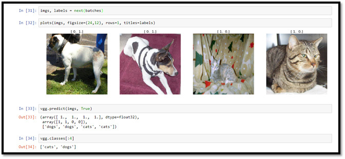
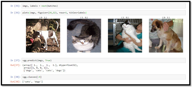
Illustration-11: 8 sample images, passed to the generated model to predict whether they are dogs or cats.
The recently announced NVIDIA Jetson TX2 for edge computing for example (which I am exploring now), is the suitable example of hardware-based embedded GPU-equipped platform in which we can deploy generated model, to be attached to a smart flying drone for example.
The Neural Network, Environment Setup
Illustration-11 shows how one component fits within the others in our environment setup.
Several frameworks and libraries are installed in the server. The important ones are Keras deep learning framework, theano deep learning library for scientific computing, and anaconda for python framework. Keras is supporting tensorflow deep learning library also, if we want to use this instead of theano.
Illustration-12 shows configuration file of keras. If we want to change the backend from theano to tensorflow, then we need only to change this file. We can change this file for keras to use tensorflow by modifying the json file content to be: “image_dim_ordering”: “tf” and “backend”: “tensorflow”. Basically change the “th” to “tf”, and “theano” to “tensorflow.”
We are using python programming language as a common language being used by data scientists worldwide; as well as jupyter notebook, the interactive environment for developer to experiment. In order to use jupyter notebook, the jupyter notebook server needs to be started as shown in illustration-6, then we can access the server at defined IP address with the assigned port: 8888. Of course other programming languages can also be used: such as Scala or R for example, depending on the needs of what we are going to accomplish.
Training (typically 60-70% of data set) & testing (typically 30-40% of data set) are very important in this supervised learning. Supervised learning means that we give a set of inputs with the set of valid outputs, then let the machine build the model (find the right mix of weights) to find a way to generate that set of outputs. The right data sets determine the quality of our generated model. In our case, there are 23,000 images in training data set and 2,000 images in testing (validation) data set.
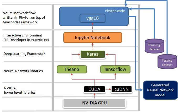
Illustration-12: vgg16.py neural network flow on top of keras libraries.
Keras is the wrapper (deep learning frqmework) for theano neural network scientific computing or tensorflow multiple GPUs neural network libraries. Both theano & tensorflow communicate to NVIDIA GPU parallel processing hardware through NVIDIA’s provided application programming interface: CUDA and cuDNN.
