Mixup data augmentation

I’ll go on details about the new modules of fastai_v1 tomorrow but before this, I wanted to spend a bit of time on a data augmentation technique called Mixup. It’s extremely efficient at regularizing models in computer vision, from what I’ve seen, allowing us to get our time to train CIFAR10 to 94% on one GPU to 6 minutes. The notebook is here, and we’ll be releasing a full conda environment to reproduce the results on a p3 instance soon (basically: you need libjpeg-turbo and pillow-simd).

What is mixup?

As the name kind of suggests, the authors of the mixup article propose to train the model on a mix of the pictures of the training set. Let’s say we’re on CIFAR10 for instance, then instead of feeding the model the raw images, we take two (which could be in the same class or not) and do a linear combination of them: in terms of tensor it’s

new_image = t * image1 + (1-t) * image2

where t is a float between 0 and 1. Then the target we assign to that image is the same combination of the original targets:

new_target = t * target1 + (1-t) * target2

assuming your targets are one-hot encoded (which isn’t the case in pytorch usually). And that’s as simple as this.

dogorcat

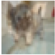
Dog or cat? The right answer here is 70% dog and 30% cat :wink:

As the picture above shows, it’s a bit hard for a human eye to comprehend the pictures obtained (although we do see the shapes of a dog and a cat) but somehow, it makes a lot of sense to the model which trains more efficiently. One difference I’ve noticed is that the final loss (training or validation) will be higher than when training without mixup even if the accuracy is far better, which means that a model trained like this will make predictions that are a bit less confident.

Implementation

In the original article, the authors suggested three things:

  1. Create two separate dataloaders and draw a batch from each at every iteration to mix them up
  2. Draw a t value following a beta distribution with a parameter alpha (0.4 is suggested in their article)
  3. Mix up the two batches with the same value t.
  4. Use one-hot encoded targets

Why the beta distribution with the same parameters alpha? Well it looks like this:

beta

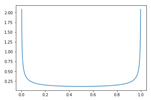
so it means there is a very high probability of picking values close to 0 or 1 (in which case the image is almost from 1 category) and then a somewhat constant probability of picking something in the middle (0.33 as likely as 0.5 for instance).

While this works very well, it’s not the fastest way we can do this. The main point that slows down this process is wanting two different batches at every iteration (which means loading twice the amount of images and applying to them the other data augmentation function). To avoid this slow down, we can be a little smarter and mixup a batch with a shuffled version of itself (this way the images mixed up are still different).

Then pytorch was very careful to avoid one-hot encoding targets when it could, so it seems a bit of a drag to undo this. Fortunately for us, if the loss is a classic cross-entropy, we have

loss(output, new_target) = t * loss(output, target1) + (1-t) * loss(output, target2)

so we won’t one-hot encode anything and just compute those two losses then do the linear combination.

Using the same parameter t for the whole batch also seemed a bit unefficient. In our experiments, we noticed that the model can train faster if we draw a different t for every image in the batch (both options get to the same result in terms of accuracy, it’s just that one arrives there more slowly).
The last trick we have to apply with this is that there can be some duplicates with this strategy: let’s say or shuffle say to mix image0 with image1 then image1 with image0, and that we draw t=0.1 for the first, and t=0.9 for the second. Then

image0 * 0.1 + shuffle0 * (1-0.1) = image0 * 0.1 + image1 * 0.9
image1 * 0.9 + shuffle1 * (1-0.9) = image1 * 0.9 + image0 * 0.1

will be the sames. Of course we have to be a bit unlucky but in practice, we saw there was a drop in accuracy by using this without removing those duplicates. To avoid them, the tricks is to replace the vector of parameters t we drew by

t = max(t, 1-t)

The beta distribution with the two parameters equal is symmetric in any case, and this way we insure that the biggest coefficient is always near the first image (the non-shuffled batch).

All of this can be found in the mixup module, coded as a callback. The bit that mixes the batch is in MixUpCallback, and the bit that takes care of the loss is in MixUpLoss (that will wrap a usual loss function like F.cross_entropy if needed). The final mixup function is in the train module, to deploy this in one line of code when needed.

53 Likes

So how effective has mixup been in your experience? It seems similar to dropout but instead of setting the value to 0 you are setting it to another value from a random picture and it happens during the data transform process.

1 Like

Hi there,
Thanks for this post!
Have you tried mixup with anything else but classification?
I wonder if you can get any benefits from this in object detection or so. Intuitively I don’t think so, but if you have tested this I would love to hear what you have found

It has proved very powerful as a regularization technique (which also means you can reduce dropout, weight decay…)

Yes, I’ve tried it in NLP, mixing the outputs of the embedding layers and it has given good results. Hoping to have time to experiment with this more and write a paper about it when the development of fastai_v1 slows down a bit :wink: I think it would also be helpful in tabular data (again mixing the embeddings fro categorical variables), not sure about object detection since I don’t see how you mixup the targets (which is critical in making mixup work properly).

12 Likes

Such an interesting idea. It reminds me a little of BPR loss, where rather than predicting a target you predict the difference between targets, but that’s in the loss, not the input. Interesting idea mixing the output of embeddings, particularly for tabular data. I’m working on a paper right now on tabular data and I think we’ll try this out and add it to the ablation.

2 Likes

@sgugger I’ve thought about this a little more and at least in the context of classification I’m surprised that it produces the linear translations between classes that the paper suggests. Unless I’m misunderstanding or getting mixed up somewhere. In my head the softmax should be creating an exponential relationship for the translation. At the end of the day it sounds like it works quite well, so I’m excited to explore it in practice, but I’m trying to understand the implications if any of this exponential relationship, or if I’m somehow wrong.

I think the use of the beta distribution might be important there, @Even, but having said that, I think you’re right - tweaking the activation to be a mixture of two softmaxes may be better still.

Can I group tabular data by category variable, then with each group I mixup continous variable. Do you think it works?

1 Like

I think that’s what Sylvain is suggesting. Treat each variable independently and do the mix on the embeddings. For continuous variables I think you just mix them directly.

How is the ground truth label when mixup two images from different classes?
And what does “the target” mean, please?

1 Like

@Gopeth see the paper:

https://arxiv.org/abs/1710.09412

1 Like

Thank U,I’ll read the paper first.

reading the code of Mixup calback, I see that the booleans:

    stack_x:bool=False
    stack_y:bool=True

are hard-coded, and for my particular classification problem where my target is (bs, number_classes) I can’t understand this line:

if self.stack_y:
            new_target = torch.cat([last_target[:,None].float(), y1[:,None].float(), lambd[:,None].float()], 1)

Computing sizes:
cat( [ (bs, n_clases, 1) (bs, n_classes, 1) (bs, 1)] ) does not work for me.
Why it is not just the weighted sum?

Ok, I understood something, I should use y_stack =True for Classifications and for multilabel should be y_stack=False.

It is missing some .float() calls, submited a PR.

2 Likes

I’ve been reading and testing the mixup model this evening but are a bit confused. In the example in the fastai documentation it trains a model with and without mixup and compares the result. Using mixup seems to make the loss larger and accuracy lower for the same number of epocs. It does the same for my image-dataset. But the paper shows otherwise. Do I have to change other regularisations like lowering dropout and weight decay to get the benefit?

I am blown away by mixup’s elegance and simplicity.

However, the implementation as described glossed over an important issue, which perplexes me. In a classification problem, labels are discrete. But a convex combination of discrete labels is not a discrete label. Thus, applying mixup transforms a classification problem into a regression problem, since it maps discrete target labels to a continuous space. Have I misunderstood something?

Instead of forming a convex combination of a pair of one-hot encoded labels

y_i,y_k

it is more natural (to me) to form convex combinations of their softmax probabilities, then assign labels by thresholding (using empirical thresholds for each class). In this way, we could handle classification problems where the target is allowed to have multiple labels.

Suppose the labels can have N classes. If the softmax probabilities for examples i and k are

\{P_{i1}, P_{i2}, ...P_{iN}\}, \{P_{k1}, P_{k2}, ...P_{kN}\}

Applying the mixup mapping, we get softmax probabilities

\{P_{mixup}\} = \{P_1, P_2, ..P_N\} = \\ \{\lambda P_{i1} + (1-\lambda)P_{k1}, \lambda P_{i2} + (1-\lambda)P_{k2}, \lambda P_{iN} + (1-\lambda)P_{kN}\}

where

\lambda

is drawn from the beta distribution

\beta(\alpha,\alpha)

and, according to the empirical studies presented in the paper

\alpha = 0.4

Next, we would determine the label(s)

y_{ik}

of the mixup example from its softmax probabilities

\{P_{mixup}\}

by applying the appropriate thresholding.

@Even and @jeremy is this is what you meant in your previous comments?

2 Likes

Cant the one hot encoded labels(only 0 and 1) already be interpreted as the softmax probability targets? Apply the convex combination will yield something like 0.3,0.7 like in the very post which seems fine to me if im not missing anything?

@Even Can you explain " In my head the softmax should be creating an exponential relationship for the translation"? I’m just interested with respects to image classification mostly.

Anyone gotten good results with the technique? This reminds of Bengio’s talk where to says that neural nets project all the inputs onto a linear space where the inputs all lie on a flat plane and a combination of them yields another valid input : https://youtu.be/Yr1mOzC93xs?t=975 . If anyone can explain what he is saying it would help us understand why mix up works better.

Yes, there should be 2 softmaxes, or something similar.

Hey Joseph,

You’ve described my thought process much more elegantly than I could have. I think @jeremy is exactly right, and that it should be a mixture of two softmaxes in the targets, although I think his earlier comment regarding the fact that this is drawn from a beta distribution is also important as most samples will have a dominant class.

Combining the images and loss in a linear way may also be helping with regularization. In the majority of cases one of the classes is dominant, and relative to it’s signal the other class is adding some noise to the input and targets sampled from the other classes. In order to get the correct scores the signal from this secondary class has to be much stronger which to me intuitively sounds like it would make the network more robust and better able to differentiate between classes. Maybe noise is the wrong term, but you get the idea.

It’s such an interesting paper/concept. One of my favourites of the year.

3 Likes

Interestingly in Amazon’s latest paper titled “Bag of Tricks for Image Classification with Convolutional Neural Networks” they used mixup to get an additonal percentage point on their CV models

2 Likes