Mean average precision (mAP)

No, no I keep the counts of TP/FP separate by classes. It’s just that I’ve read some people presenting the algorithm to count them with watching the hits on ground truth object but I think they might sort them by decreasing overlaps, so the big dog and big sofa boxes are matched with ground truth sofa (bigger IoU), but not the ground truth dog.

So it’s a bit clearer with a (short) night of sleep. In the end I let myself be confused by the matching process (how to attribute a prediction to a ground truth object) which is kind of the same as in the loss function.

I’ve update the notebook to fix some bugs, get a bit more efficient and added a lot of visualization of TP/FP/FN in the hope it will help people that are as confused as I were. I’d be curious to see if my final mAP is correct or not, so any feedback is more than welcome!

4 Likes

Hey, thanks again for sharing and updating your notebook! Great stuff and useful learning for me, especially on making things readable and more computationally efficient.

I’ve been (very slowly) coding my way to a fuller understanding of TP, FP, and FN scoring, adjusting the model and IoU thresholds, all the way to mAP (correctly I hope).

For reproducibility and consistency across our work, I copied the first half of your notebook and loaded your trained weights (thanks for that!) to start off at the same point. I hope by the end, I’ll be able to tell you that our mAPs match up (or at least why they don’t).

For now, I wrote some new visualization/educational functions to count every TP, FP, FN, and ground truth object for every class category in an image so I could play around with the model sensitivity and IoU thresholds. Along with some commentary, it looks like this:

Here is my adapted nb: https://gist.github.com/daveluo/2ab83da32e623864e543d7251e9beef4

Hope it’s helpful. I’m moving steadily but slowly on implementation so will continue to comment as I go!

2 Likes

Thanks for your comments! We already disagree on one situation so I’m not sure we’ll find the same results, in his image:

I’m counting
sofa : 1TP
dog: 1FP, 1TN
because the predicted box of the dog is matched to the ground truth object sofa in my code since it’s the one it overlaps the most but it might be mistake.

Aaaaah! Got it!
I forgot we have to detect TP,FP and FN for each class separately! So you’re right and I’m wrong on this one. Will try to correct my functions tonight or tomorrow.

2 Likes

Thanks for the follow-up! I was scratching my head too and checking if I misunderstood something somewhere (among the incredibly confusing amount of materials about mAP…)

To lay out my current understanding using the dog and sofa example in the image:

For class ‘dog’:

  1. calc jaccard(all ‘dog’ predictions, all ‘dog’ gt_bboxes)
  2. for all ‘dog’ predictions where IoU > 0.5 (or a different iou_thres), take the highest IoU box and call that TP (more generally: for n ‘dog’ ground truth objects, count n-highest IoU ‘dog’ predictions as TPs)
  3. count all other ‘dog’ predictions as FP. If all predictions for the class are <= IoU threshold, then they’re all counted as FPs? This last part I’m not too sure on yet…

Repeat for class ‘sofa’ and any other class of interest.

For mAP more generally, we loop through all classes one at a time. Even if there’s no ground truth objects in a class, we still want to catch all false positive since a prediction could be made for a class outside of ground truth (i.e. a prediction for ‘car’ in our example image would be a FP in ‘car’ class). We also want to catch all false negatives in every class (i.e. if a ‘sofa’ gt object has no predicted boxes, that would be a FN in ‘sofa’ class).

Does that sound right to you?

Btw, I’ve created a P-R curve up for category 14 (‘person’) using a range of model thresholds = np.linspace(.05, 0.95, 40, endpoint=True) which I believe is the same as your nb.

Shape looks pretty similar despite the difference of TP/FP/FN counting. I guess because across the whole image set, it’s not a significant difference in the P or R calcs:

pr_cat14

The AP of cat 14 in this P-R curve (using your avg_prec func) comes out to be 0.286.

2 Likes

Yes, it’s all clearer to me now, thanks for re-explaining it because it sure needs the details.
I’ve finished rewriting the functions to (hopefully) have the same results as you in terms of TP/FP/FN and updated it on github. In the end, I get to 0.2863 for the AP of class 14 and it changes the whole mAP from 30.7% (bugged version) to 30.99% (new version) so it was indeed small.

Hope this last version is the good one!

1 Like

Awesome! I’ve also finished running the full 40-step range of model thresholds on all 20 categories. Ended up with a mAP of 30.17%. I guess the full description of the metric result should be “mAP@ 0.5 of 20 classes using 11-point interpolated average precision” to be exacting.

I’ve updated my gist as well. The code is painfully inefficient, needs refactoring, and I want to double check to see why we have a 0.8% diff in our mAPs.

Here are my P-R curves per class (with APs on top). If you could generate something similar, comparing them will probably be the quickest way to spot any major class-specific discrepancies between our methods:

Update: I had a list of mAP benchmarks here but I don’t think they’re up to date (mAP ranged from 22.7-43.7 and newest paper was from 2013). Here’s the performance table from the SSD paper:

It’s not immediately clear to me what the exact mAP performance criteria they use is…my homework for tomorrow morning :slight_smile:

2 Likes

Great discussion in this thread!

Maybe comparing results to the MultiBox paper might be a better idea.

Not sure how to best verify the correctness of the implementations of mAP :thinking: Maybe a pretrained model for one of the archs exists and we could run it to output predictions and calculate the mAP?

Other than that probably implementing quite faithfully one of the simpler models and comparing the results might be the best proxy.

Will most likely get around to doing such a thing myself but given the pace at which I am going someone is very likely to beat me to it :slight_smile:

Anyhow, having a working implementation of mAP that we can trust would be quite cool!

1 Like

Here are the figs with my version of the code

The difference between our scores (and figs) is the way we treat the zeros in TP+FP or TP+FN. I chose to put one when we have 0/0 to have nicer curves, not sure of what is the right way it should be done.

If I take the same function as you do for the precision and recall (by adding 1e-15 to the denominator) I get 30.17% as well.
I don’t think they took this definition of mAP in the SSD paper. Ours is the one that used in the 2007 competition and I think the formula changed in the evaluation for 2012. And I didn’t check but it might also be different for the COCO dataset/competitions.

1 Like

Mystery solved, and quickly too! Thanks for checking and making the figs.

I added an epsilon number of 1e-15 to avoid ZeroDivisionError. Looking at the public implementations of mAP, one of them sets precision=0 if there’s a division error and two of them (including the official cocoeval.py) uses the smallest possible epsilon (np.spacing(1) = 2.220446049250313e-16) either as an addition to TP+FP or as max(TP+FP, eps).

I’ll change my treatment of division errors to that last approach (max(TP+FP, eps)) which seems most appropriate and remove eps from the recall calculation where it’s unnecessary (assuming there’s always at least 1 gt object present of every class across the full test set).

This change won’t do much for our mAP though. I’ll do some manual checking, particularly within the poorer performing classes like ‘sheep’ and ‘boat’, and see if there are any steps amiss between individual image TP,FP,FN scoring and P-R curve construction.

I also came across this paper, “Diagnosing Error in Object Detectors”, which is frequently cited. It does confirm that we are counting our TPs and FPs correctly with regards to the IoU threshold >0.5.

Informative further break-out of the types of FP errors:

One major type of error is false positives, detections that do not correspond to the target
category. There are different types of false positives which likely require different
kinds of solutions. Localization error occurs when an object from the target category
is detected with a misaligned bounding box (0.1 <= overlap < 0.5). Other overlap
thresholds (e.g., 0.2 <= overlap < 0.5) led to similar conclusions. “Overlap” is defined
as the intersection divided by union of the ground truth and detection bounding
boxes. We also consider a duplicate detection (two detections for one object) to be localization
error because such mistakes are avoidable with good localization. Remaining
false positives that have at least 0.1 overlap with an object from a similar category are
counted as confusion with similar objects. For example a “dog” detector may assign
a high score to a “cat” region. We consider two categories to be semantically similar
if they are both within one of these sets: {all vehicles}, {all animals including person},
{chair, diningtable, sofa}, {aeroplane, bird}. Confusion with dissimilar objects
describes remaining false positives that have at least 0.1 overlap with another labeled
VOC object. For example, the FGMR bottle detector very frequently detects people
because the exterior contours are similar. All other false positives are categorized as
confusion with background. These could be detections within highly textured areas
or confusions with unlabeled objects that are not within the VOC categories.

2 Likes

I’ve taken a tour through the lowest scoring AP classes (all < 0.100) : ‘sheep’, ‘bottle’, ‘boat’

Doing so leads me to believe our mAP calculations are essentially correct (with minor quirks like handling division by zero differently) and a roughly accurate reflection of our model performance. Taking a look at the worst performing classes also helped me IDed a few areas of improvement where tweaking our model architecture and training parameters should help increase mAP score.

ISSUE 1:
Our model struggles with very small, numerous gt objects like sheep. For example, let’s look at the TP, FP, and FN count of ‘sheep’ at different model threshold levels (the ‘model_thres’ value defined in NMS: c_mask = conf_scores[cl] > model_thres) with visualized prediction bboxes versus gt bboxes:

NMS CONFIDENCE THRESHOLD: 0.15
  2 FP 'bird'
  1 FP 'cow'
  0 TP, 19 FP, 3 FN, 3 actual 'sheep'

NMS CONFIDENCE THRESHOLD: 0.25
  0 TP, 5 FP, 3 FN, 3 actual 'sheep'

NMS CONFIDENCE THRESHOLD: 0.35
  3 FN 'sheep'

Across threshold levels, we generate a different number of False Positives as expected but we never get any TP hits on ‘sheep’ because the prediction box IoUs are always < 0.5. At the lower end, we have many FPs instead which reduce our Precision score and at the higher end, we stop making predictions and end up with all FNs.

Here are some other examples of this where the gt objects are very small:

NMS CONFIDENCE THRESHOLD: 0.15
  4 FP 'bird'
  1 FP 'cat'
  0 TP, 1 FP, 1 FN, 1 actual 'sheep'

NMS CONFIDENCE THRESHOLD: 0.15
  2 FP 'bird'
  2 FN 'sheep'

We have a similar problem with ‘bottle’ where they’re usually very small and/or numerous:

NMS CONFIDENCE THRESHOLD: 0.15
  0 TP, 1 FP, 2 FN, 2 actual 'bottle'
  2 TP, 13 FP, 3 FN, 5 actual 'person'

NMS CONFIDENCE THRESHOLD: 0.25
  1 FN 'bottle'
  2 FP 'chair'
  1 TP, 2 FP, 3 FN, 4 actual 'person'
  1 FN 'pottedplant'
  0 TP, 1 FP, 1 FN, 1 actual 'sofa'

ISSUE 2:
The model also struggles with narrow (very tall or wide) rectangles and/or scales that range from one extreme to another. Basically objects that aren’t as square-ish or of consistent scale…i.e. tall bottles or tall boats that take up different proportions of the image frame:

NMS CONFIDENCE THRESHOLD: 0.20
  3 TP, 4 FP, 1 FN, 4 actual 'bottle'

NMS CONFIDENCE THRESHOLD: 0.15
  1 TP, 8 FP, 0 FN, 1 actual 'boat'

NMS CONFIDENCE THRESHOLD: 0.25
  1 TP, 2 FP, 1 FN, 2 actual 'boat'
  1 FN 'person'

In these situations, it looks like we usually get our TPs but also many FPs that fail to be suppressed.

ISSUE 3
Our classes are not balanced in training (or evaluation). Some classes show up less often than others so our model doesn’t have as many examples to train on. The diversity of how objects are presented within images (small flocks of sheep in the corner vs one large main subject sheep) also affect the generalizability of training. This alone doesn’t explain performance but it should be a contributing factor. I’ve highlighted the number of ‘sheep’, ‘boat’, ‘bottle’ objects in our dataset:


from http://host.robots.ox.ac.uk/pascal/VOC/voc2007/workshop/everingham_cls.pdf

Here are some ideas to try which should help improve model mAP:

  1. Use more grid cells and more zooms to create smaller anchor boxes. Something like 7x7, 4x4, 2x2, 1x1 to capture small objects like sheep and bottles.
  2. Increase the aspect ratio parameters to have even more narrow rectangles to catch ships/bottles/people.
  3. Try stratifying train and val datasets (like what StratifiedKFold does in scikit). And/or or upsample underrepresented classes to get more class-balanced.
  4. Tweaking Non Max Suppression settings to adjust how many FPs remain.
7 Likes

Wow, thanks for the amazing summary!
The model clearly need more anchors, which is what they do in the original SSD paper. I’m trying to roughly replicate what they do (with a total of 8732 anchors!) and will share as soon as it’s ready. Maybe it will help with the narrow or the very little objects.

1 Like

This is great analysis. To add to the suggestions:

  • I’m not at all convinced the way I use tanh and turn the activations to anchor box changes is much good. It’s really just the first thing I came up with. Maybe check the yolo3 paper and see what they do, and try changing our code to do the same thing - does that help?
  • The papers don’t have different zoom levels IIRC - so they have lower k, but more conv grid outputs
  • Try making out custom head look more similar to the retinanet and/or yolo3 custom heads
  • Try using a feature pyramid network. This is what I plan for lesson 14, but I haven’t started on it yet

Overall, I’d suggest trying to gradually move our code closer to the retinanet and yolo3 papers, since they get great results so we know it should work!

3 Likes

Thanks for the additional ideas! I’m definitely planning to implement more stuff from retinanet and yolov3 and learn about FPNs so will keep posting with updates.

Now that we have working P-R curves and APs to benchmark and do more in-depth diagnostics per class and per image, it’ll be easier to evaluate if and how these changes help performance.

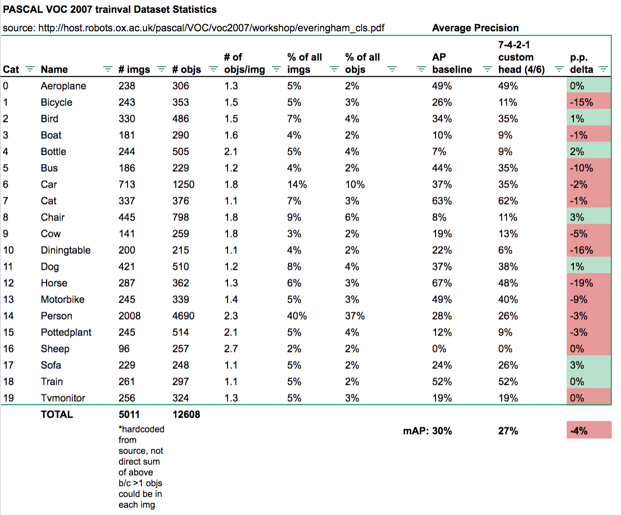
For example, I’ve been testing custom heads like using 7x7 grid cell (for more smaller anchor boxes) and different k combos to get better bbox localization and reduce False Positive rate. Haven’t been able to break our baseline mAP of 30% yet but this helps us investigate the model performance more granularly with sample images:

Or as class APs compared to baseline:

I’ve updated my gist with a lot of refactoring and computation speedup (much thanks to @sgugger for the prediction masking idea: got me from ~40mins -> 1-2mins to compute everything!). Also cleaned up the “model investigation” functions so they’re more obvious to view and use.

UPDATE:

I used these mAP metric functions to evaluate my coconut tree detector:

image
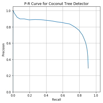
Looking pretty great! Average Precision of 74.9%

Out of curiosity, I plotted Precision and Recall on separate y-axes with the prediction confidence threshold on x-axis to visualize the P-R tradeoff as you move the confidence threshold up or down:

image

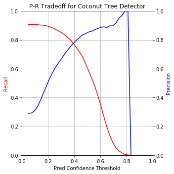
md_thres=0.4 seems like the best balance with ~80% on both precision and recall. Let’s visualize that performance on a few images:

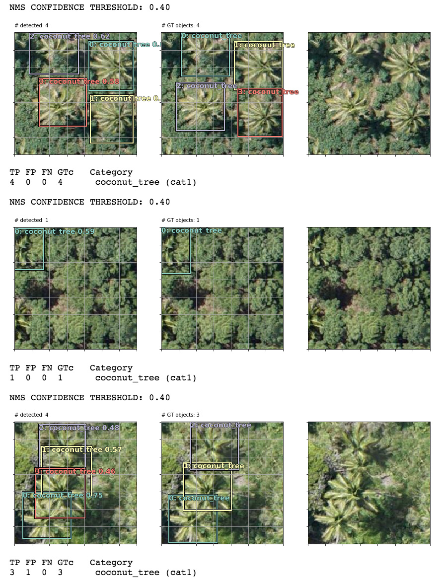
Our detector caught every TP in these 3 images. In the last image, you could make a good argument (looking at the raw image) that the 1 FP is actually a TP that was missed by human annotators.

7 Likes

I also spent some time struggling trying to master mAP concept and spent some hours analyzing the official PASCAL VOC code.

I created one repository that provides easy-to-use functions implementing the same metrics mentioned in this article (Average Precision and mAP). The results were carefully compared against the official implementations and they are exactly the same.

If anyone wants to use, here it is: https://github.com/rafaelpadilla/Object-Detection-Metrics

5 Likes

Do you calculate mAP after non-max suppression or before? As this would greatly affect the numbers of TP/FP that are used to calculated precision/recall values.

Thanks. This is another simple explanation,

I’ve read @daveluo and @sgugger’s notebooks thoroughly, and I was very surprised to see that they calculated AP by varying the predicted-class-confidence threshold. Why does that work? I can’t find any references to that method in any of the resources. It was my understanding that we had to set the class confidence threshold to around zero, including many false positives but not affecting the overall score very much (because they come in at the tail).

Here’s the image of a PR curve that Dave used above, but I’ve included the text in the article directly above it. It seems to me that this says we need to relax the class confidence threshold to near-zero to calculate mAP:

I realized that the code those gents wrote does exactly what I thought it should, but in reverse! The “textbook” method of sorting preds by conf desc to build the PR curve starts by basically finding the left-most point on the PR curve, but the method in the notebook starts by finding the right-most point.