Wow, thanks for the amazing summary!
The model clearly need more anchors, which is what they do in the original SSD paper. I’m trying to roughly replicate what they do (with a total of 8732 anchors!) and will share as soon as it’s ready. Maybe it will help with the narrow or the very little objects.
1 Like
This is great analysis. To add to the suggestions:
- I’m not at all convinced the way I use
tanhand turn the activations to anchor box changes is much good. It’s really just the first thing I came up with. Maybe check the yolo3 paper and see what they do, and try changing our code to do the same thing - does that help? - The papers don’t have different zoom levels IIRC - so they have lower
k, but more conv grid outputs - Try making out custom head look more similar to the retinanet and/or yolo3 custom heads
- Try using a feature pyramid network. This is what I plan for lesson 14, but I haven’t started on it yet
Overall, I’d suggest trying to gradually move our code closer to the retinanet and yolo3 papers, since they get great results so we know it should work!
3 Likes
Thanks for the additional ideas! I’m definitely planning to implement more stuff from retinanet and yolov3 and learn about FPNs so will keep posting with updates.
Now that we have working P-R curves and APs to benchmark and do more in-depth diagnostics per class and per image, it’ll be easier to evaluate if and how these changes help performance.
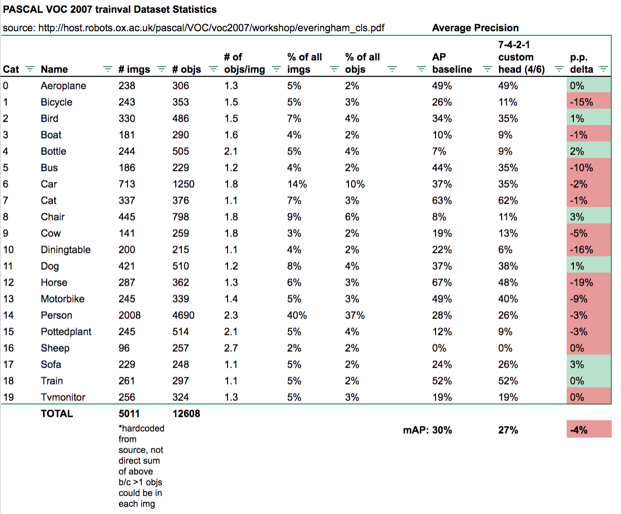
For example, I’ve been testing custom heads like using 7x7 grid cell (for more smaller anchor boxes) and different k combos to get better bbox localization and reduce False Positive rate. Haven’t been able to break our baseline mAP of 30% yet but this helps us investigate the model performance more granularly with sample images:

Or as class APs compared to baseline:
I’ve updated my gist with a lot of refactoring and computation speedup (much thanks to @sgugger for the prediction masking idea: got me from ~40mins -> 1-2mins to compute everything!). Also cleaned up the “model investigation” functions so they’re more obvious to view and use.
UPDATE:
I used these mAP metric functions to evaluate my coconut tree detector:
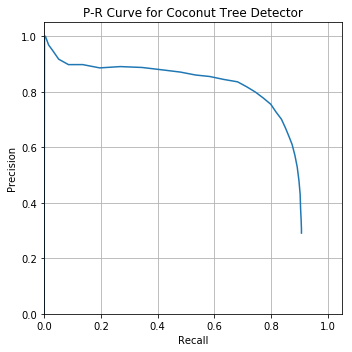
Looking pretty great! Average Precision of 74.9%
Out of curiosity, I plotted Precision and Recall on separate y-axes with the prediction confidence threshold on x-axis to visualize the P-R tradeoff as you move the confidence threshold up or down:
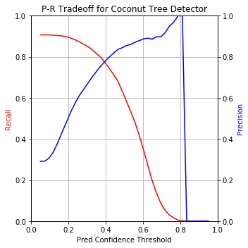
md_thres=0.4 seems like the best balance with ~80% on both precision and recall. Let’s visualize that performance on a few images:
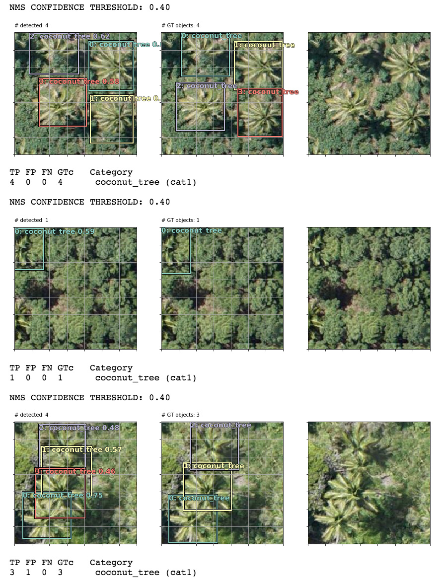
Our detector caught every TP in these 3 images. In the last image, you could make a good argument (looking at the raw image) that the 1 FP is actually a TP that was missed by human annotators.
7 Likes
I also spent some time struggling trying to master mAP concept and spent some hours analyzing the official PASCAL VOC code.
I created one repository that provides easy-to-use functions implementing the same metrics mentioned in this article (Average Precision and mAP). The results were carefully compared against the official implementations and they are exactly the same.
If anyone wants to use, here it is: https://github.com/rafaelpadilla/Object-Detection-Metrics
5 Likes
Do you calculate mAP after non-max suppression or before? As this would greatly affect the numbers of TP/FP that are used to calculated precision/recall values.
Thanks. This is another simple explanation,
I’ve read @daveluo and @sgugger’s notebooks thoroughly, and I was very surprised to see that they calculated AP by varying the predicted-class-confidence threshold. Why does that work? I can’t find any references to that method in any of the resources. It was my understanding that we had to set the class confidence threshold to around zero, including many false positives but not affecting the overall score very much (because they come in at the tail).
Here’s the image of a PR curve that Dave used above, but I’ve included the text in the article directly above it. It seems to me that this says we need to relax the class confidence threshold to near-zero to calculate mAP:

I realized that the code those gents wrote does exactly what I thought it should, but in reverse! The “textbook” method of sorting preds by conf desc to build the PR curve starts by basically finding the left-most point on the PR curve, but the method in the notebook starts by finding the right-most point.