Two goals for this post:
- Share a potentially useful little tool for accumulating multiple loss traces (from multiple runs of lr_find, for example)
- Share some experiences with lr_find using this tool, and see if this is consistent with others’ experience or expectations.
I started reading the paper by Leslie Smith on tuning hyper-parameters (which I believe was the inspiration for lr_find), and I was struck by the idea of comparing multiple runs of lr_find with different settings of other hyper-parameters. I ginned up a tool to let me do that (link above), and got this plot (note it is zoomed in to focus on the inflection points):
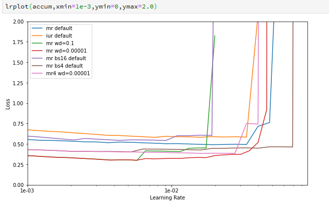
In this figure I can see some variation in how much learning happened, and where the learning rate gets too great, across several variations of weight decay and batch size. But how significant are these variations? How much variation is to be expected just by the randomness of the process?
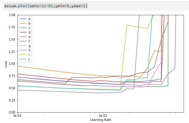
So I tried a different experiment: redo the same lr_find 10 times, on the same model but different data selected at random. Here’s the code and the resulting plot :
accum = infra.LRAccumulator()
for i in range(10):
    tr_list, val_list = windows.randomer_split(allwindows)
    learner = zoo.MultiUResNet.create(tr_list, val_list, title="randomer multiresnet", bs=8)
    learner.lr_find(neptune=False)
    accum.add(learner)
accum.plot(xmin=1e-03,ymin=0,ymax=2)
(Side note: I have a lot of custom code for building my models and datasets, but hopefully the loop is pretty comprehensible anyway, and none of the custom stuff should affect the results.)
The conclusion from the plot is pretty clear: the variation in the second chart is easily as great as the first. So I don’t think I can conclude anything about the different hyper-parameters from the first graph. Moreover, the data you get from a single run of lr_find (at least with my model and data) has a span of about an order of magnitude when showing you the turning point in the learning rate.
Then I redid the same experiment above, but with a much longer/slower lr_find process (setting num_it=1000). Here is the output of that experiment:
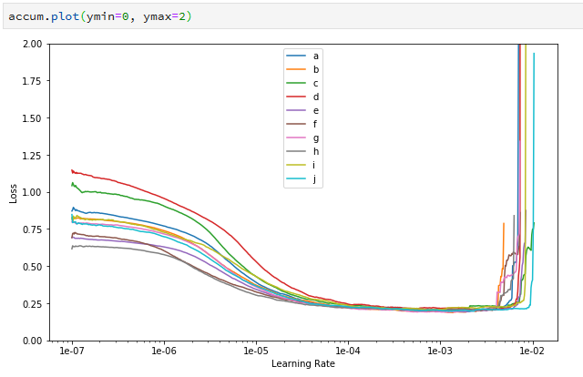
In this case I’m showing the entire x range rather than focusing just on the inflection points. There are a couple of interesting observations from this graph, compared with the previous ones:
- Even though the losses started off differently on the different runs, they all converge very tightly. This might mean that you could use this longer lr_find process to effectively distinguish the overall effect of hyper-parameters on loss rate. More work TBD.
- The inflection point still has a pretty broad spread, though (it’s about half the width of the previous one).
- Perhaps most interestingly, the inflection point has moved left by almost an order of magnitude. My gut guess is that this might have something to do with the fact that the loss has converged/flattened before the inflection point was hit.
So thoughts I’m pondering:
- How much is this dependent on my specific data/model? I’m really just at the beginning of my model-building process and there’s a pretty good chance that the model itself will need to be improved before I get anywhere. Would lr_find be more consistent on a better model?
- Is the lr_find default iteration count (num_it=100) too low? Or maybe should we run lr_find a couple of times and take an average?
What do other folks think — what is your experience with using lr_find?
(FWIW: the problem space I’m looking at is multi-class segmentation with multispectral Landsat data. The code is in my repo here, but I haven’t come up with a good way to publish/share the data yet.)