Lesson 9 official topic

[puru]

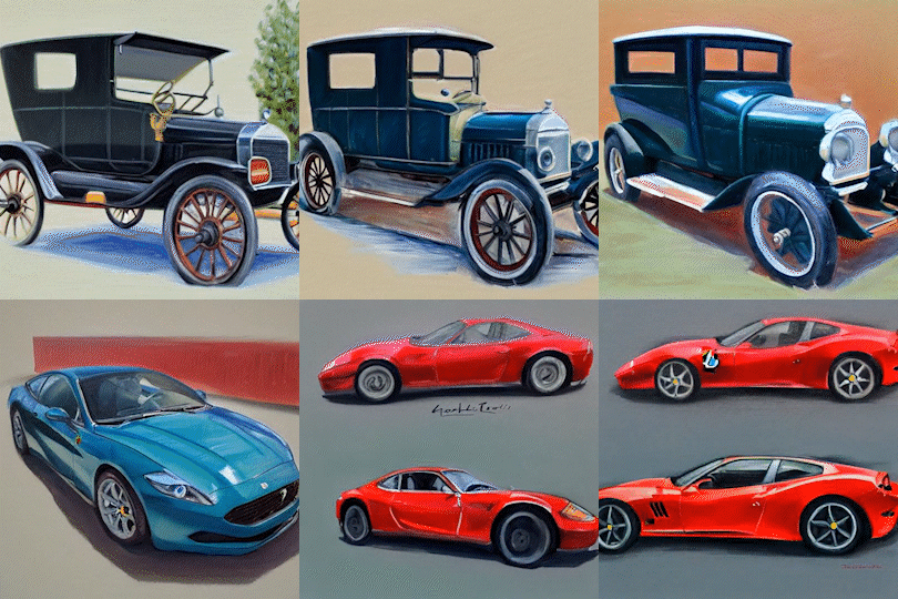
i made a jupyter nb that interpolates between prompt embeddings as well as noise latents. created this animation that shows the evolution of a Ford Model-T to a Modern-day Ferrari

link to the nb: here
ported from nate raw’s gist