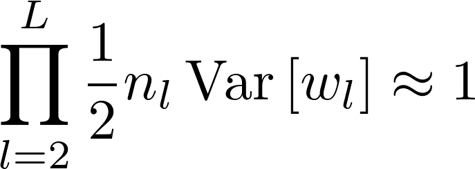
One thing i observed is that at the end of section 2.2. Kaiming mentions that that both forms observed in forward-prop and backward-prop are equivalent and would be sufficient to ensure that we initialize properly.
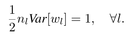
First form in forward prop is
∀l,12nlVar[wl]=1
backward prop is
∀l,12n̂ lVar[wl]=1
n̂ l = (kl) ^ 2 * dl
nl = (kl)^ 2 * d(l-1)
This ratio can either be diminishing or exploding. I am not sure if it can be neither unless it is 1 and in the paper also it has been mentioned that this isn’t diminishing. But i’m not sure if that isn’t exploding either.
This also means that the ratio of weights across the layers is perhaps important.
For convolutions the quotient is number of number of output channels divided by the number of input channels. When you multiply those up, you have the number of channels at the beginning divided by the number of current channels. For resnet, the maximum number of channels is 512.
If you are terribly concerned, you could add a hook (PyTorch activation.register_hook(lambda x: x*my_factor)) between the layers to multiply the gradient by n̂/n, but as pointed out here, some of the other assumptions are more an ideal setup to reason about than exactly true.
I don’t know if the question belong in this thread, but does anyone know if correlated features (inputs) would make the problem of exploding gradients worse? If not, are you aware of any other issues it might cause, or in general DNN don’t care about input correlation?
I did some Google search and didn’t get any clear answer one way or another.
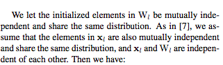
I think so. In particular, your assumption about about the independence of the activations is false:
Likewise, the elements in x_l are mutually independent and share the same distribution.
Remember, the x_l are not randomly initialized. This is most obvious in the first layer: we can rescale the inputs but that doesn’t cause them to be independent. x_{l; i} in later layers will be calculated from the same inputs in earlier layers (although with different weights) – hence won’t be independent.
It’s actually not my assumption, it’s made in the original Kaiming paper (that itself took it from the Xavier paper):
I agree that the independence of the activations is questionnable. Interesting that that equation still holds only with the uncorrelated assumption though, I didn’t think about that.
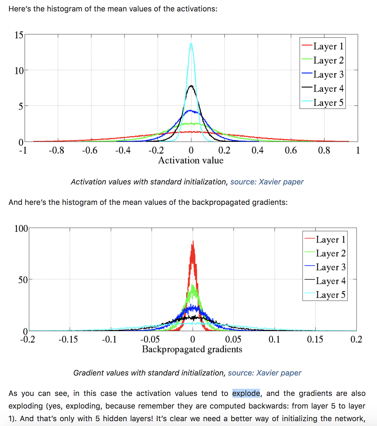
Real basic question. Can someone explain to me how these plots show the activations/gradients exploding?
To me it looks like vanishing. In the forward pass (going from layer 1 to 5), the mean activation values converge to 0 (or the 0-peak, using the terminology from the paper). Similarly in the backward pass (going from layer 5 to 1), the backpropagated gradients converge to 0.
I think you’re very right and I’m wrong. I read it as a graph with values of the activations on the y-axis, but I went too fast and it’s actually an histogram. Thank you for spotting this
I think the reason why the layer std is around 0.8 in the notebooks is the following (I don’t know why it would be decreasing in later layers though).
Kaiming-He isn’t trying to make sure that the variances of the post-relu layers are equal to 1, just that they are equal across all layers (so they don’t explode or vanish). So they will all be equal to the variance of the first layer activations.
In their notation,
Var[y_l] = n_l Var[w_l] \mathbb{E}[x_l^2]
But on the very first layer, \mathbb{E}[x_1^2] = 1 (assuming the inputs are normalized), so if we use Kaiming-He initialization, the first layer pre-ReLU will have std \sqrt2.
If the pre-ReLU std is \sqrt2 , then the post-ReLU std. will be ~0.825. Around the same as in the notebook.
(The reason for the latter claim is that the normal distribution has a lower conditional variance. For example, for a standard normal, the std conditional on being larger than 0 is ~0.58. Numbers taken from:
import numpy as np
np.random.seed(1)
x = np.random.normal(size = int(1e7))
y = np.maximum(x, 0)
x.std(), y.std(), y.std()*np.sqrt(2)
How do you expand the expectation of the max function? I think it’s in the way I wrote below, but I am not sure. Could you please clarify if that is correct? Since the max function is piecewise defined, I expanded the expectation of the max function as probability-weighted expectations of the pieces, but I am not sure if that is correct and such rule of expansion even exists (I tried to Google for expectation of the max function but the answer uses scary integrals and doesn’t explain in a clear way). I would be grateful for clarification:
Since y_{l-1} is distributed symmetrically around 0, it’s positive half the time and negative half the time (symmetrically!), so if just keep the positive part max(0, -), you’re keeping half of the expectation. More explicitly, you can break the expectation up into when y_{l-1} is negative and when it’s positive.
Anyway, the two integrals are the two pieces you’re looking for (the “rule of expansion” you refer to). It’s just splitting up an integral into two pieces.
I was looking into pytorch implementation of these initializations and found that in order to calculate the bounds of uniform distribution, they multiply the standard deviation by square root of 3.
fan_in, fan_out = _calculate_fan_in_and_fan_out(tensor)
std = gain * math.sqrt(2.0 / (fan_in + fan_out))
a = math.sqrt(3.0) * std  # Calculate uniform bounds from standard deviation
with torch.no_grad():
    return tensor.uniform_(-a, a)
I wonder where that sqrt(3) came from. I can’t find anything about this relationship between normal and uniform distribution. I will appreciate if someone explain that or point in right direction.
This also came up in the study group at USF, so maybe you shouldn’t be kept waiting…
The \sqrt{3} comes from the standard deviation of a uniform distribution – if you select uniformly from [-a,\,a], the standard deviation is a/\sqrt{3}. (You can look it up from Wikipedia, but why is that the answer? – a question Jeremy posed the study group)
kaiming_uniform tries to solve the opposite problem: if a uniform distribution on [-a, \,a] has a standard deviation std (from your code snippet above), what is a? (That’s why the \sqrt{3} is in the numerator, rather than the denominator.)
This doesn’t have anything to do with normal distributions, by the way.
Ok, now i see where that came from. If you calculate the formula of std for uniform distribution on the interval [-a, a] you will get \frac{a}{\sqrt{3}}. Since \sigma^2 = \frac{(b-a)^2}{12} : \sigma = \sqrt{\frac{(\alpha - (-\alpha))^2}{12}} = \sqrt{\frac{(2\alpha)^2}{12}} = \sqrt{\frac{4\alpha^2}{12}} = \sqrt{\frac{\alpha^2}{3}} = \frac{\alpha}{\sqrt{3}}
I believe I have sensible initialization of my layers, but since I am using a pre-trained embedding as a first layer, how can I control the standard deviation after that step?
I have checked and the mean activation is close to 0, but standard deviation after embeddings (for a given text) is a bit over 3!
(The rest of the layers have nicer std values, ranging from 0.35 after some convolutions to close to 1 for the final layers.)
This works but it is not the only way to solve the equation (e.g. 0.8 * 1.25 is also 1). Did the authors choose to make every multiplication equal 1 because it was easier? Can we expect some difference in performance if we selectively initialize different layers to different scales while conserving the overall multiplication = 1?