Let’s say you have a class Linear that has a __call__ method. Then you can use that method like so: Lin()(). The first () calls the __init__ and returns an instance. The second () calls __call__ on that instance.
6 Likes
I think for einsum the order of input indices in that string doesn’t matter, it will figure out the order automatically based on the output. This is why it is so easy to use einsum, you don’t need to think about order. So both your cases work just the same.
2 Likes
Great lesson, as Jeremy mentioned there is a lot to learn and experiment.
I wondered about this too, but I think this is because we are actually doing an outer product (from the code above in the nb):
def backward(self):
        self.inp.g = self.out.g @ self.w.t()
        # Creating a giant outer product, just to sum it, is inefficient!
        self.w.g = (self.inp.unsqueeze(-1) * self.out.g.unsqueeze(1)).sum(0)
        self.b.g = self.out.g.sum(0)
I think “b” stands for batch in the einsum. In the example this is 50,000.
So in the first layer we have:
50000 x 784  -->  50000 x 784 x  1
50000 x 50   -->  50000 x   1 x 50
Here “i” is 784 and “j” is 50. In the end we get 784 x 50 before we do the row sum.
And in the second linear layer we have this.
50000 x 50  -->  50000 x 50 x 1
50000 x  1  -->  50000 x  1 x 1
I believe einsum is just hiding the unsqueezing details. Can someone else confirm this?
2 Likes
This was cool!
Quick question: Can we think of the .clamp_min(0.)-0.5 as essentially a version of Leaky Relu?
Afaik you can use with einsum any variable naming and there is not a specific reserved variable, i.e., b is not necessarily the batch dimension.
This is a great PyTorch einsum tutorial:
https://rockt.github.io/2018/04/30/einsum
5 Likes
No. It’s more a “shifted relu”. In a leaky relu, you have a (small) slope in the negative range, while here you don’t (but have a small negative activation).
1 Like
It looks like this: max(x,0)-0.5 for x from -1 to 1 - Wolfram|Alpha
4 Likes
Monday morning up before 6.00 am, sorting out my platforms for part2 etc plus shopping for vitals. Very busy all day. Thought I would fall asleep during lesson, but fixed on every word from 1.20 am to 4.00am on the 19th. Not sure if it was meant to be top down or bottom up, to me it was top down in the sense that the accelerator continued to the floor.
Regards for that inspirational insight jph00.
4 Likes
On one of the first slides of lesson 8 Jeremy shows the 2 steps for model training:
- Overfit.
- Reduce overfitting.
I completely agree with Jeremy’s definition of overfitting: “the condition when the validation loss starts to increase”, but this condition does not necessarily imply that our model has captured the complexity of the underlying function.
Even a very simple model can overfit in that sense. In the context of model training, I think we aim for both overfitting (as defined above) and also strongly reducing training loss so we are sure we can at least reproduce the training target. Then we can start #2 - namely try to reduce the overfitting model.
Any thoughts?
3 Likes
I think from a "loss landscape" point of view, overfitting means that the model is stuck at a local minima, probably a sharp one. The training loss might not be low enough since its just a local minima. These local minima might be your usual saddle points.
However in case of a sharp local minima, the training loss may actually get quite low. This does not mean that the loss is low when tested on the validation set, since the loss landscape for the validation set might be high at that point. Like explained by Jeremy in the Fastai-v2 lesson 2:
Hence, we can say that the training loss is sometimes misleading. From a practitioner’s point of view, validation loss serves as a more reliable indicator of overfitting.
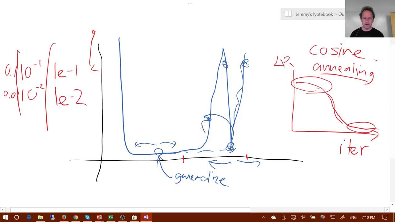
Now that we are sure that our model is overfitting (validation loss is not reducing anymore), we can take some steps to rectify this situation (escape this minima). Jeremy explains how learning rate annealing can escape the sharp minima shown above. Similarly, batch normalization also helps reduce overfitting by smoothening the loss landscape:

As we can see that after batch normalization the sharp local minimums have reduced significantly and the model can now roll onto greener pastures downhill.
Hence, the two steps:
- Overfitting till validation loss does not reduce anymore (stuck at local minima)
- Reduce overfitting through regularization (escape the local minima)
Does anybody else have any other explanation or a better intuition that they are willing to share?
1 Like
An minor but important correction to both of the above - it’s the accuracy we want to track, not the loss. Remember we discussed in part 1 that your accuracy will keep improving even after your loss starts getting worse. Trying to really understand why that is, is an excellent way to deepen your understanding of model training. 
(Also, I don’t think over-fitting finds sharp local optima. I think they’re actually wide local optima, but in bad parts of the loss surface.)
12 Likes
If you want to copy a tensor that requires grad, you’ll need to do .detach().clone() yes.
2 Likes
Looking forward to batch norm …would be nice to have some mention of “conditional batch norm” too, I found the latter illuminating in thinking about batchnorm is as this odd statistical mini network / architectural add-on.
1 Like
I’m not the authority by any means on this but have also done part 2 v2.
From the looks of it, they’re adopting a very different methodology this time, going from the ground up code wise and learning all the tricks needed while showing how to do it efficiently, with the use case of building a library. So I reckon, it’ll be worth it.
It won’t be as useful from learning different applications perspective but I believe this will allow for more people to build what they want as they’ll have all the necessary tools.
1 Like
Did anyone catch what day the study group was? This was in the slides but it didn’t mention the days.
- Room 153 @ USF 101 Howard St
- Generally someone is there 10am - 4pm
3 Likes
I replicated the Excel file in a Google sheet (including steps on how to do it). So, everyone can access it. 
16 Likes
Why guess when we can experiment? ![]()
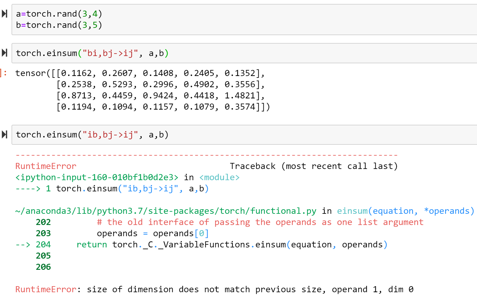
So order of indices absolutely does matter. Which makes perfect sense really - since it’s the order of indices that defines how each axis maps to the output.
4 Likes
As I briefly mentioned in class, I’m trying to give you all enough material to keep you busy until the next course. So don’t worry if it doesn’t all make perfect sense right away - take your time to go through the code, experiment, and read additional external resources on those areas that interest you or you feel you need to fill in some gaps. ![]()
7 Likes
We already spend quite a bit of time on randomized linear algebra in the Computational Linear Algebra course taught by @rachel.
All the interesting things I have to say about optimization I’ll be saying in this upcoming course. ![]()