I spoke to my ISP but they require me to get a static/public IP (Sorry If I’m mixing 2 terms here) so that I can allow incoming traffic, so I’m forced to purchase the add on
Thank you! I ended up setting up noip, it was a hassle free setup, just a few adjustments were required on my router (Most routers turns out have a DDNS option in-built).
Sorry to steer the discussion off Lesson 8, but is it suggested to run just scripts on the machine instead?
Based on the suggestions above, I’m doing the following:
Setup SSH on my “box”.
Put the public key of my laptop on the ssh folder in the “box”
Enabled ssh services in Ubuntu
Enabled port forwarding of port 22 (internal) to Port 22 (External) on my router
Thanks for the clarification.
Don’t know why '__call__' came as a '__custom__'def in my head, my bad.
Notes:
__call__ makes a instance of a class callable as a function.
class model:
    def __init__(self, arg1, arg2, arg3):
     # code
    def __call__(self, arg1):
    # code

resnet = model(foo1, foo2, foo3) #instance of a class

resnet(image) #making it a callable (instance as a function)
resnet.__call__(image) #is same as above
Here __init__ is basically a constructor, as it is invoked once by __new__ when the object is created , but __call__ can be called with the object any number of times which gives us the flexibility to redefine it (like, changing the state).
Also, in a deep learning setting the state of an entity (for example, layer) changes after each iteration. Some of the framework(design) decisions in pytorch makes a lot of sense now.
Wait, now I’m a bit confused – does it really matter whether you use the training set or the validation set? It does seem like in practice the distributions should be very similar, but I thought the point you were trying to make in class was that both the training set and validation sets should be normalized in a consistent manner.
Perhaps it’s slightly suboptimal for training to normalize the training set using the validation set (you will no longer be guaranteed to be training on a set that has mean 0 and stdev 1), but it seems minor compared to normalizing the training and validation sets independently.
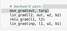
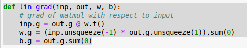
Yeah, I get these mixed up too—I always have to go back and rederive things with explicit indices in the chain rule and then see if I can spot the matrix multiplications afterwards. Is there an easier way? I guess just memorize some matrix derivative identities? Probably time to work through the matrix calculus post
As an example, for calculating the derivative of the loss with respect to weight W_{ij} from a linear layer y_{nj} = \sum_i x_{ni} W_{ij} + b_j (here n is the batch index), I’d have to do the following: W_{ij} affects the loss via y_{nj} for every n in the batch (but not via any of the other activations for some index other than j), so if we already know all those upstream derivatives \partial \mathcal{L}/\partial y_{nj} (aka out.g), then the chain rule gives
and yeah, if I squint I can write that as a matrix multiplication as x.t() @ out.g.
I actually kind of like all the explicit indices (otherwise I tend to forget things like the batch index), and I think it makes the chain rule a little easier to feel than with the matrix notation, but it’s definitely a little tedious…
Here is a short answer I can come up with. torch.randn gives you random numbers of specified shape whose mean is 0 and standard deviation is 1. We want our input and activations to have mean 0 standard deviation 1; not the weight matrix.
Edit: woops, didn’t search hard enough in the thread, @mkardas was way ahead of me
Random thought about the shifted ReLU idea: the avg. value of a standard normal truncated to be positive is 1/\sqrt{2\pi} (about 0.4), so what about doing ReLU - 1/\sqrt{2 \pi} rather than ReLU - 0.5? Lol presumably that doesn’t do much different, but it looks cool
For whatever it’s worth, the shifted/renormalized ReLU interacts with Kaiming initialization in a strange way. Eq. 7 from the paper
Var[y_l] = n_lVar[W_l]E[x_l^2]
uses the fact that E[x_l^2] = \frac{1}{2}Var[y_{l-1}], when the activation is ReLU, to obtain their initialization scheme. But if we shift ReLU by c, then
When c = -0.5, for example, the extra terms come out to be 0.25 - E[y_{l-1}^+].
So it probably depends on how your input data is distributed, but if e.g. the E[y_l^+] > 0.25, then the variances of your later layers are probably going to be less than that of your earlier layers compared to if you had used plain ReLU. For example, as it’s been pointed out a few times in this thread, if we assume the y_l are N(0,1), then E[y_l] = \frac{1}{\sqrt{2\pi}} \approx 0.4.
The intuition behind doing things in batches is that 1 input is not enough to know to right “direction”, so you take multiple inputs and assume that the (averaged) gradient will take the step in the right direction.
Over 1 epoch, you take lots of steps ( ~[number of inputs / batch size] steps), each in the direction of the averaged gradient of the current batch.
Thanks @PierreO. I do get the logic, but if I am not mistaken, in the notebook the sum is used, hence my question. I always thought we use the average of gradient for each batch to the backprop.
I don’t think there’s any need to explicitly average gradients—you just calculate the loss, which is usually implicitly averaged across the batch, e.g. the “mean” in MSE. That happens in some of the notebooks when we divide by some shape[0] (the batch dimension).
This is a hard concept to really “get it”. I think this is what’s explained in 4.4 of https://arxiv.org/pdf/1802.01528.pdf and after reviewing partial derivative and reading that section many times, it still doesn’t sink in fully.