trying to get behind RL scepticisim I sometimes hear in the community. While I am not competent enough to judge and have no real opinion, this here seemed interesting: https://thegradient.pub/why-rl-is-flawed/ @gmohandass
great class, indeed ! need to go through this again too.
Working thru the notebok 01_matmul I tried this:
`c1 = tensor([[1],[2],[3]])`
`c2 = tensor([[1,2,3])`
c1,c2
(tensor([1],
[2],
[3]),tensor([[1,2,3]]))
c3=c1+c2;c3
tensor([2, 3, 4],
[3,4,5],
[4,5,6]])
but :
c4 = c1.expand_as(c2)
fails with:
RuntimeError: The expanded size of the tensor (1) must match the existing size (3) at non-singleton dimension 0. Target sizes: [1, 3]. Tensor sizes: [3, 1]
so there’s more going on here than just the expand_as before the tensor operation.
Hi, I might be wrong but if you compare equation of sigmoid vs RELU its is big difference in complexity.
Computer do very fast adding and shifting bits other operations are very expensive RELU do pretty good job and id very easy to compute
Right - read the ‘broadcasting rules’ section to see what actually happens.
I am not sure if that is what is really happening, but this would be my take on this:
As we continue to train our model, it becomes more confident in it’s predictions (for a classification problem, the outputted values grow closer to 0 and 1). Overall, the model is doing a better job at classifying images (accuracy keeps increasing) while the loss grows as well. That is because for the now fewer examples that are misclassified, as the model becomes more confident in its predictions, the loss increases disproportionately.
If we look at how the cost is calculated using cross entropy, the more wrong the model is (difference between predictions and ground truth approaches 1) the cost asymptotically approaches infinity IIRC. So the few misclassified examples count by a lot.
Now, I don’t think this could happen if we were considering all examples in the dataset during training. But as the loss is calculated on a batch of examples, the model can still be learning something useful, becoming better overall, while we see an increase in loss (though here we probably only care about the validation loss so that is a slightly moot point).
EDIT: The image below is showing the effect:
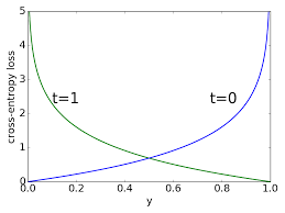
For a positive class, notice how little the cost grows from a predicted probability of 0.6 to 0.4. For as long as the model operates in that middle ground the cost changes slightly. But observe the explosion in cost as the predicted probability approaches 0!
Image taken from these lecture slides returned by google search.
That’s the key insight!
What happens is that for the start of training, the model gets better at predicting, and more confident (correctly) of those predictions, so accuracy and loss both improve.
But eventually, additional batches only make it slightly more accurate, but much more confident, such that that over-confidence causes loss to get worse, even as accuracy improves.
Since what we actually care about is accuracy, not loss, you should train until accuracy starts getting worse, not until loss starts getting worse.
I’ve just added them to the top post of this topic.
This article has also a nice visualization and explanation for broadcasting: https://jakevdp.github.io/PythonDataScienceHandbook/02.05-computation-on-arrays-broadcasting.html
Hi fellow students,
I started with the matmul implementations as discussed in the lesson and found few interesting things that I would like to share. I also came across some observations which needs your review/help, they are marked as TODO in the notebooks.
Update: tagging @sgugger for help
I will share my interpretation. Please, correct me if there’s something wrong: What we really want to track is the metric, not the loss function. We use the gradient of the loss instead of the metric for updating the weights because the loss is better behaved. On the other hand, the metric provides a “human readable” value that allows us to judge how good or how bad is the model. However, in regards to this part:
Remember we discussed in part 1 that your accuracy will keep improving even after your loss starts getting worse.
Can anyone point me which lesson was this behaviour observed? In my mind, the loss and the metric would somehow have a correlation. For example, in regression problems, R2 score is just a normalized version of MSE.
Does anyone know how much research has been done into S-shaped RELU activations? That is:
-k if x < -a, k if x > a, else x (or other versions)
This would also have a zero mean.
First hit I found was this which shows positive results, but fairly old network architectures: https://arxiv.org/pdf/1512.07030.pdf
You are right, I did not pay attention to bi
and ib
part. What I meant is that the order of input arrays doesn’t matter (while it does matter for regular matrix multiplication with @
or matmul
)
For order of the arrays, einsum
will figure it automatically (of course it is a different thing and not what was asked in the original question):
Very good insights. Thanks for sharing
Was torch.tensor out of bounds or why did we use fastai’s tensor command instead of going directly to torch. Is there a benefit of using that command? Here is the line I’m talking about:
x_train,y_train,x_valid,y_valid = map(tensor, (x_train,y_train,x_valid,y_valid))
I would have instead used :
map(torch.tensor, (x_train,y_train,x_valid,y_valid))
(and let’s be honest I would have done each of those individually, who knew that map was a thing?)
Looked into the fastai tensor command a bit more and it looks like it actually uses torch.tensor so I’m guessing that is ok to use.
Is there a way to see the code of a built-in function or method?
I was going to look at what exactly torch.randn does to generate its random numbers with a normal distribution, but ??torch.randn
doesn’t seem to work. It gives me the documentation but not the code.
torch.randn??
So the takeaway would be whenever you’re making a tensor of n similar iterables or applying a function to n iterables, just replace that with 1 single line of map(YourFunc, n1, n2....n)
Actually if you check the import section:
from torch import tensor
Which is why we can type tensor instead of torch.tensor
For other functions, if you look at the online PyTorch docs, there is an option that shows us the source code, but for torch.randn the same isn’t there either.
I’m not sure why it behaves this way, but for ?tensor
and ??tensor
and same for the randn function, both just return the docstring.
Thoughts on Lesson 8
This post summaries my ideas after the lesson and centres around these
elements.
- Normalisation
- Bayesian Methods
- Augmentation
Normalisation
The idea of normalising the data has significant weight in this lesson.
What we have done is normalise continuous variables, what would a
normalised categorical variable look like, would it be the same or not?.
Would this approach be readily applied to other learning strategies e.g.
- RandomForest Regression/Classifier
- GradientBoosting
- RandomTreeEmbedding
If we subject our data to mean of 0 and stdev of 1 then Bayesian methods
can be applied?.
Bayesian Methods
The figure below is taken from [^1] And it is a figure of a hierarchical
model taken from Chapter 3 Modeling with Linear Regression it shows a
series of distributions to make up a regression y = \alpha + X \beta
Augmentation
Given that we can create regressions from distributions and there are discrete
distributions for categories see [^1] could this be used for augmentation i some
way
I appreciate I may not have explained this very well but I am sure some discussion will help.
[^1]: Bayesian Analysis with Python Second Edition Author Osvaldo Martin
[^1]
Any idea on what rtol and atol means in the below code
torch.allclose(a,b,rtol=1e-3,atol=1e-5)