For the number of factors is there a way to determine the number of factors we should consider or is there a good rule of thumb to start? I guess how did we come up with 5 as a number of factors to work with?
http://yaoyao.codes/python/2016/09/25/python-starred-expression
Important to know for the *self.y_range piece of the forward method.
Edit: Forgot the most important part:
def sum(a, b):
return a + b
values = (1, 2)
s = sum(*values)
1 Like
Thanks for a great lecture.
2 Likes
Truthfully, I generally suggest looking at what other people are doing in competitions and such as your starting points, or just try it yourself. I have done it a few times and I think it is just experience. I think 5 may be small, so that it would be easy to visualize. (long time since I have looked at recommendation systems)
1 Like
@sgugger thank you for that reply. So what that means is that you’d go through your dataset and label something like this: image1: 90% person, 60% animal; image2 30% person, 88% animal, etc.
That’s the general idea, if I understand you. But what would a practical example of an actual label like that be? A label like “man” or “woman” doesn’t mean anything to a computer if you’re doing a classification problem (it could be “homme” et “femme” or for that matter “pollywog” and “skittle” as long as these labels were attached to images of men and women, respectively). But if I want to show something more fine-grained, like degree of importance, what would the label actually look like?
Also how many items would need to be labeled like this to have this work – if you had person, animal, and bicycle, would the number needed go up more?
i had a hard time understanding the different input shapes - and why the architecture sill works - too  . I think I figured out how it works - if im wrong please let me know
I built a Conv1d Resnet for inputs like Audio Files and first had the problem, that when the length of the input (audio-file) changed, I had to adopt the network architecture. Watching one of Jeremys other lessons (GAN from 2018 I think) he mentioned the difference between the different pooling layers (Average pooling vs adaptive average pooling especially). Using AdaptiveAvgPool*d does the trick .
Heres an easy example for Conv1d with 1 input dimension (mono audio). I printed the shapes after each layer / resnet block to understand how the shapes change. And this example is a lot easier to understand compared to Conv2d with 3 input dimensions (RGB images). Because the tensors have just 3 dimensions [batch_size, number_output_kernels, “length”] instead of … a lot dimensions 
Heres a 1 second 24414 hz mono audio [bs 64, 1 input channel, length: 24414 samples]:
in torch.Size([64, 1, 24414])
in conv torch.Size([64, 16, 24414])
in bn torch.Size([64, 16, 24414])
l1 torch.Size([64, 16, 24414])
l2 torch.Size([64, 32, 6104])
l3 torch.Size([64, 64, 1526])
l4 torch.Size([64, 128, 382])
l5 torch.Size([64, 256, 96])
l6 torch.Size([64, 512, 24])
avgpool torch.Size([64, 512, 1])
You can see, that the number of kernels increases (16 to 512) - that’s defined by your network architecture:
        self.conv = conv1x3(1, 16)
        self.bn = nn.BatchNorm1d(16)
        self.relu = nn.ReLU(inplace=True)
        self.layer1 = nn.Conv1D(block, 16, kernel_size)
        self.layer2 = nn.Conv1D(block, 32, kernel_size, stride)
        self.layer3 = nn.Conv1D(block, 64, kernel_size, stride)
        self.layer4 = nn.Conv1D(block, 128, kernel_size, stride)
        self.layer5 = nn.Conv1D(block, 256, kernel_size, stride)
        self.layer6 = nn.Conv1D(block, 512, kernel_size, stride)
        self.avg_pool = nn.AdaptiveAvgPool1d(1)
The last dimension changes according to the length / size of the input (from 24414 to 24 in the first example).
Now here’s a 0.75 second Audio clip with 18310 samples.
in torch.Size([64, 1, 18310])
in conv torch.Size([64, 16, 18310])
in bn torch.Size([64, 16, 18310])
l1 torch.Size([64, 16, 18310])
l2 torch.Size([64, 32, 4578])
l3 torch.Size([64, 64, 1145])
l4 torch.Size([64, 128, 287])
l5 torch.Size([64, 256, 72])
l6 torch.Size([64, 512, 18])
avgpool torch.Size([64, 512, 1])
you can see that the last dimension as the size of 18 here.
Now the trick: Adaptive Average Pooling will calculate the average of the tensor over the last dimension (independent of the size!) and will reduce it to 1 (nn.AdaptiveAvgPool1d(1) as specified here). Thats why the input shape doesn’t matter for (this kind of) CNNs.
5 Likes
Thanks for this man.
I was about to dive into the same exercise for a very simple CNN and I will report back on my findings.
Admittedly, the AdaptiveAvgPool detail had flown over my head, and it makes sense.
I guess the critical part is the model’s head, e.g. when you switch from Conv to densely connected layers as this is when your matrix multiplication will fail, so I agree that AdaptiveAvgPool seems to iron out any potential shape discrepancy.
Let me try to figure this out with a very basic CNN and will let you know.
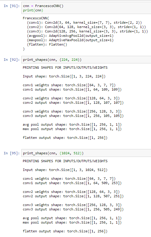
@florianl I replicated your experiments with a very basic CNN.
You are totally right that AdaptiveAvgPool2d is the key.
Look below how the CNN can process squared or rectangular images without problems.
I guess this closes the issue
from torch.nn import Conv2d, Module, AdaptiveAvgPool2d, AdaptiveMaxPool2d, Flatten

class FrancescoCNN(Module):
    def __init__(self):
        super(FrancescoCNN, self).__init__()

        self.conv1 = Conv2d(3, 64, kernel_size=7, stride=(2, 2))
        self.conv2 = Conv2d(64, 128, kernel_size=3)
        self.conv3 = Conv2d(128, 256, kernel_size=3)

        self.avgpool = AdaptiveAvgPool2d(output_size=1)
        self.maxpool = AdaptiveMaxPool2d(output_size=1)
        self.flatten = Flatten()

    def forward(self, x):
        x = self.conv1(x)
        print(f'conv1 weights shape: {self.conv1.weight.data.shape}')
        print(f'conv1 output shape: {x.shape}\n')

        x = self.conv2(x)
        print(f'conv2 weights shape: {self.conv2.weight.data.shape}')
        print(f'conv2 output shape: {x.shape}\n')

        x = self.conv3(x)
        print(f'conv3 weights shape: {self.conv3.weight.data.shape}')
        print(f'conv3 output shape: {x.shape}\n')

        x = self.avgpool(x)
        print(f'avg pool output shape: {x.shape}')

        x = self.maxpool(x)
        print(f'max pool output shape: {x.shape}\n')

        x = self.flatten(x)
        print(f'flatten output shape: {x.shape}\n')
        return x

def print_shapes(net, size):
    print('PRINTING SHAPES FOR INPUTS/OUTPUTS/WEIGHTS')
    x = torch.Tensor(1, 3, *size)
    print(f'\nInput shape: {x.shape}\n')
    _ = net(x)
3 Likes
No, that’s not how you would want to label, assume you want to classify if an image has a man and/or a horse. Then you would have to give samples man, horse and a third category of man and horse.
Correct the value attribute to label doesn’t actually matter to the model, as you have seen in the bear classifier, the classes gets converted to number ( technical term would be one hot encoding, covered in lesson today)
Can you please elaborate on this one?
Like we have seen in earlier examples, with transfer learning, you can do well with less items, even as less as 20 items per class, you can check the projects done by students in earlier course for this.
Provided that the items are representative of the test data you will be running the inference with.
Hope this clarifies.
Yes! my GTX-1080 does fp16, but it’s not faster than fp32
2 Likes
Here’s another data point. For my vision applications (cnn: resnet, densenet),
I have a 2080 ti, on a ubuntu 18.04 machine. 16fp trains faster (~15%) than 32fp.
They can be anywhere you like, but your get_x function will have to make the path for them.
This is sometimes referred to as “lazy loading.” It’s used in a lot of frameworks to make sure that data arrives just-in-time, and of-course to preserve memory.
@sgugger – nevertheless, @giacomov’s suggestion makes sense to me – i.e. for each learning rate, average the loss over several mini-batches.
No expert here, but you’re probably going to have to modify the dataloader classes you use to load the X data to read your additional columns (in addition to the flattened RGB image. Example: a 3x3 pixel image has 9 pixels values between 0-255 for each of 3 (RGB) channels for a total of 27 x values per row, now if you added time (lets say), you’d be adding a 28th value to the row.
Hey guys, I could use some help here: I’ve been reading the Cyclical Learning rates paper and in describing the triangular learning rate policy this code is given:
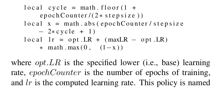
Now the paper says that the variable epochCounter is the number of epochs of training which means that the cycle variable is only going to increase to say 2 when the number of epochs is greater than or equal to 2*stepsize. So for a stepsize of 2000, we would have to train for 4000 epochs or more before the cycle increases from 1 to 2.
However, I think that the epochCounter should rather refer the number of iterations which I think would make more sense.
@sgugger @muellerzr
Yeah, the equation is wrong. There’s a post about it
https://forums.fast.ai/t/draft-of-fastai-book/64323/39
But I didn’t see a reply to that person’s post.
1 Like
Anyone having issues running the notebook for collaborative filtering on the merge part?
ratings = ratings.merge(movies)?
I changed the name, but even with “movies” it won’t work. any suggestions?
---------------------------------------------------------------------------
MergeError                                Traceback (most recent call last)
<ipython-input-34-eb862f217676> in <module>
      1 #issue in merge
----> 2 ratings = ratings.merge(scripts)
      3 ratings.head()

/opt/conda/envs/fastai/lib/python3.7/site-packages/pandas/core/frame.py in merge(self, right, how, on, left_on, right_on, left_index, right_index, sort, suffixes, copy, indicator, validate)
   7295             copy=copy,
   7296             indicator=indicator,
-> 7297             validate=validate,
   7298         )
   7299

/opt/conda/envs/fastai/lib/python3.7/site-packages/pandas/core/reshape/merge.py in merge(left, right, how, on, left_on, right_on, left_index, right_index, sort, suffixes, copy, indicator, validate)
     84         copy=copy,
     85         indicator=indicator,
---> 86         validate=validate,
     87     )
     88     return op.get_result()

/opt/conda/envs/fastai/lib/python3.7/site-packages/pandas/core/reshape/merge.py in __init__(self, left, right, how, on, left_on, right_on, axis, left_index, right_index, sort, suffixes, copy, indicator, validate)
    618             warnings.warn(msg, UserWarning)
    619
--> 620         self._validate_specification()
    621
    622         # note this function has side effects

/opt/conda/envs/fastai/lib/python3.7/site-packages/pandas/core/reshape/merge.py in _validate_specification(self)
   1196                             ron=self.right_on,
   1197                             lidx=self.left_index,
-> 1198                             ridx=self.right_index,
   1199                         )
   1200                     )
MergeError: No common columns to perform merge on. Merge options: left_on=None, right_on=None, left_index=False, right_index=False
Why are the points, from the chapter 6 regression example, normalized to a value between -1 and 1?
I understand that is why we use the y_range we do … but I’m not sure why that range to being with.
learn = cnn_learner(dls, resnet18, y_range=(-1,1))
When we do points it’s converted to a %, -100% (far left) and +100% (far right), with 0,0 at the very center of the image. Does this help @wgpubs? it makes augmentation much easier as everything is now relative vs other libraries that struggle with point augmentation
1 Like