Lesson 5 official topic

@wyquek thanks for offering to help. Unfortunately, passing act=lambda x:x has no effect on the results.

I am stumped as to why these predictions don’t just work out-of-the-box.

1 Like

Solved!!

I went through the fastai source code for learn.predict() and realized that this code was wrong

dl_test = TextDataLoaders.from_df(df, valid_pct = 0, text_col='text', shuffle=False)[0]
predicts, actuals = learn.get_preds(dl = dl_test)
predicts

This code does work. If there is a more idiomatic way to do this, please let me know.

model = "ulmfit.pkl"
learn = load_learner(model)
dl_test = learn.dls.test_dl(df.text.to_list())
predicts = learn.get_preds(dl = dl_test)
predicts

Out[93]:
(TensorText([[3.1701e-04, 9.9968e-01],
         [3.8059e-02, 9.6194e-01],
         [5.1746e-01, 4.8254e-01],
         [9.6458e-04, 9.9904e-01],
         [1.0545e-01, 8.9455e-01],
         [4.6742e-03, 9.9533e-01],
         [3.9310e-01, 6.0690e-01]]),
 None)

Can you explain more? What code was wrong, and how was it wrong?

1 Like

Sorry. To be clear, I meant to say my code was wrong. The source code is fine. In fact, it was the source code that helped me figure out why learn.predict() was working for me, but learn.get_preds was not. I looked through the fastai documentation, tutorials and the forums and just wasn’t able to figure it out. I should have looked at the source source code sooner. . .

This code is wrong. Unfortunately, it didn’t fail with an error, so I didn’t recognize that I had made a mistake as I was getting back answers. Only after really looking at the results did I conclude that something was wrong.

dl_test = TextDataLoaders.from_df(df, valid_pct = 0, text_col='text', shuffle=False)[0]
predicts, actuals = learn.get_preds(dl = dl_test)
predicts

Out[307]:
TensorText([[0.8213, 0.1787],
        [0.8429, 0.1571],
        [0.8596, 0.1404],
        [0.8174, 0.1826],
        [0.8157, 0.1843],
        [0.8967, 0.1033],
        [0.8972, 0.1028]])

This code works, though I don’t know if it is idiomatic:


dl_test = learn.dls.test_dl(df.text.to_list())
predicts = learn.get_preds(dl = dl_test)
predicts

Out[93]:
(TensorText([[3.1701e-04, 9.9968e-01],
         [3.8059e-02, 9.6194e-01],
         [5.1746e-01, 4.8254e-01],
         [9.6458e-04, 9.9904e-01],
         [1.0545e-01, 8.9455e-01],
         [4.6742e-03, 9.9533e-01],
         [3.9310e-01, 6.0690e-01]]),
 None)

From what I see it looks exactly like how to use the inference API! :smile:

3 Likes

Does anyone know why we are not zeroing out the gradients after each epoch in this course notebook (Linear model and neural net from scratch | Kaggle)? This is something that is normally done during each mini-batch/step, which in this notebook - 1 step/mini-batch is one training epoch as there is only a single batch, and seems like a bug although it does not seem to negatively affect the loss and accuracy too much when training for 30 epochs, but I have noticed some other issues. Maybe it does not matter in this case because of the relatively small dataset size and relatively small number of epochs. I’m trying to figure out if this was done on purpose or is a bug.

I ran a series of experiments on the linear model both with and without coeffs.grad.zero_(). When training for 30 epochs, I was able to achieve a slightly higher accuracy 0.831460 with coeffs.grad.zero_() at epoch 19 vs 0.825842 without it (matching the accuracy in the course notebook), but the losses were consistently worse and accuracy was worse at the original final epoch (30) as well.

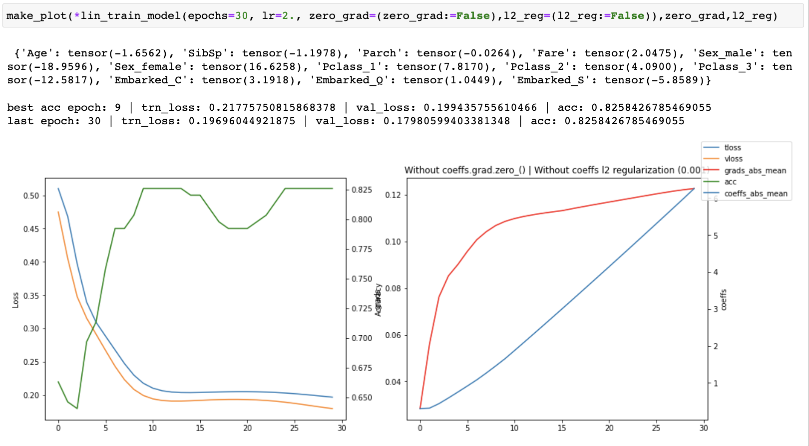
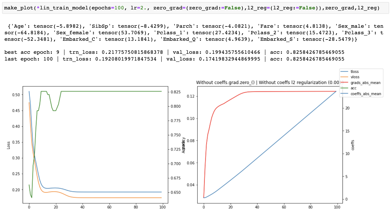
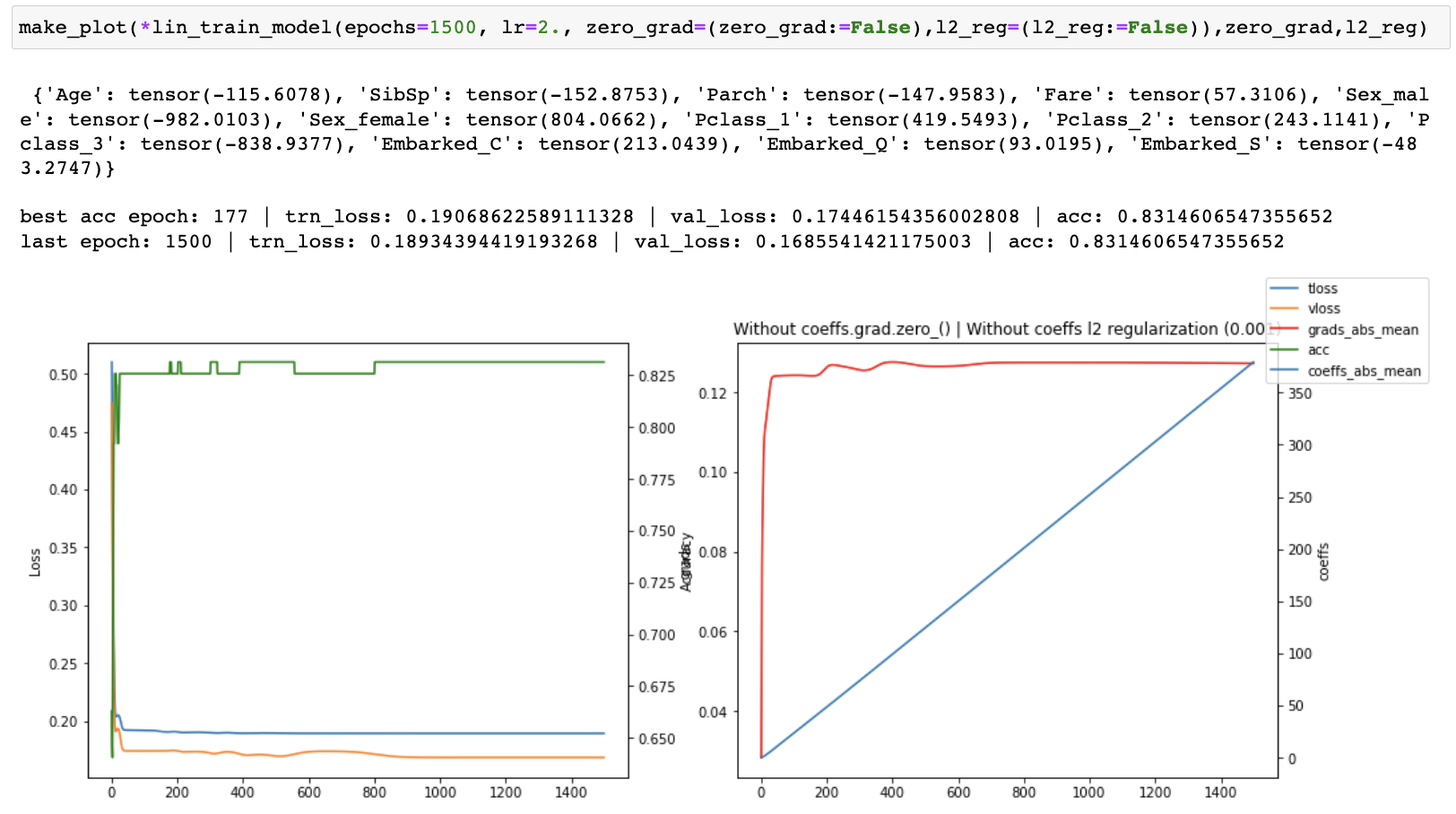
I then started tracking the losses, accuracy, gradients and coefficients and created plots of each one of them to see what was happening as training progressed. I ran both with and without coeffs.grad.zero_() for 30, 100 and 1500 epochs.

without coeffs.grad.zero_()


with coeffs.grad.zero_()


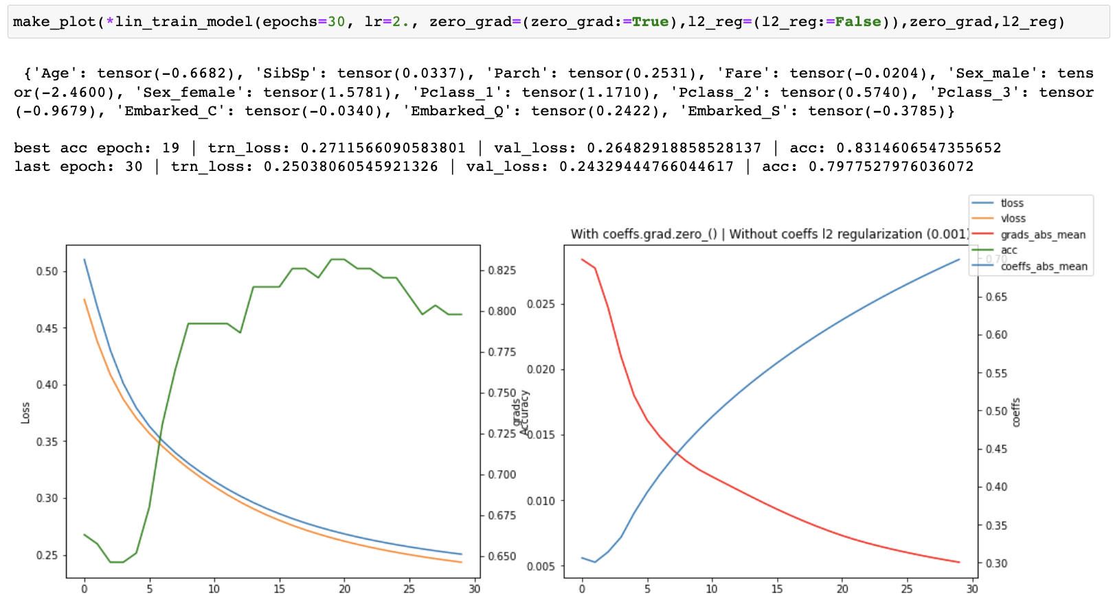
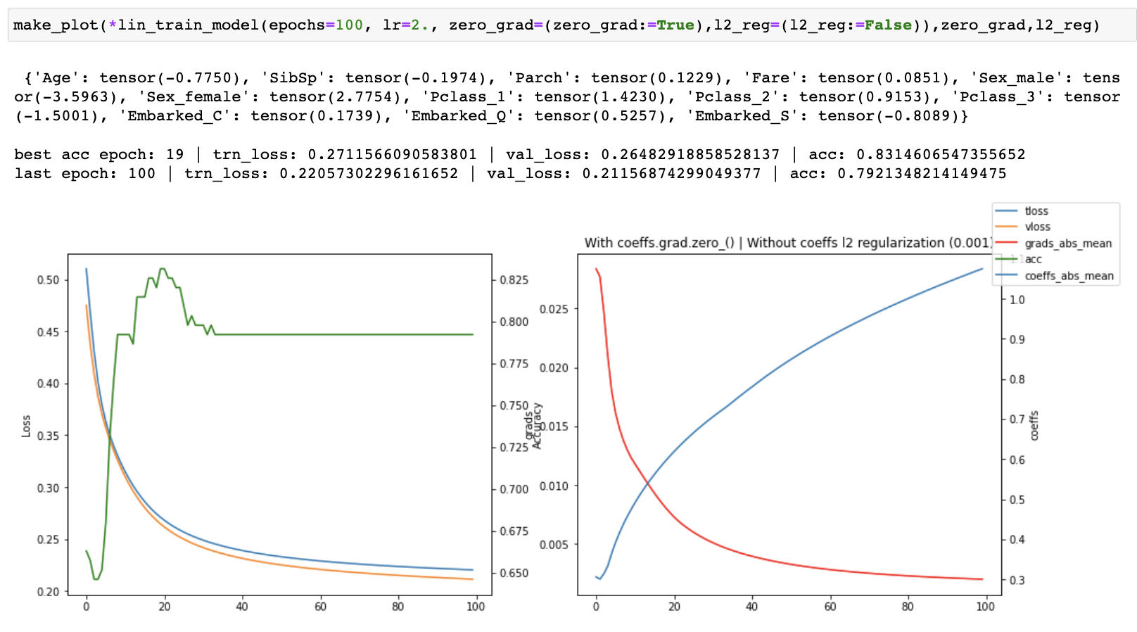
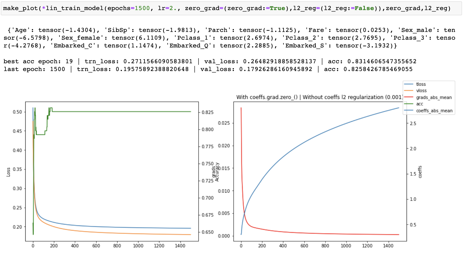
When running without zero_grad_ I noticed that the coefficients were growing linearly with the number of epochs which is not ideal. When running with zero_grad_ the coefficients were still continuously growing, but the graph of the coefficients looked like a log graph instead of a linear graph and the overall values were much lower which was much better. I then added a simple l2 regularization (ish) of the coefficients to the loss and ran some more experiments. This helped to prevent continuous growth of the coefficients.


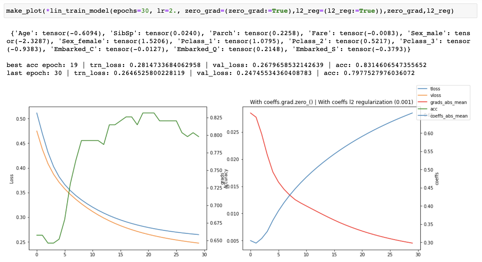
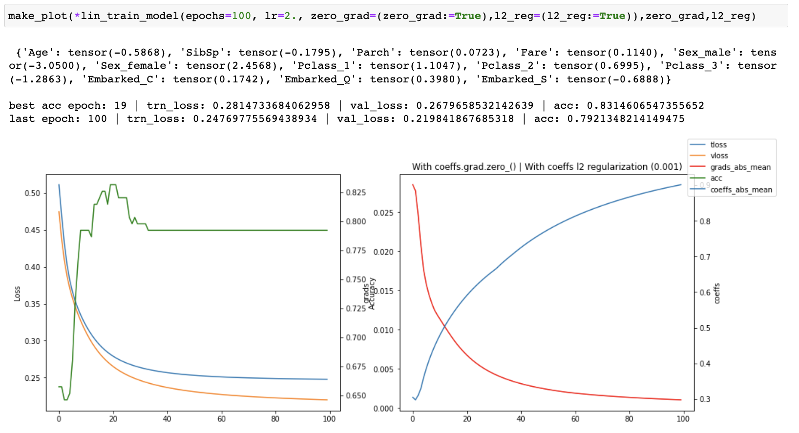
I then tried keeping the coefficient l2 reg and turning off zero_grad_ and that caused training to become unstable, even with a much lower learning rate. This happened consistently across a number of different runs with different hyperparameters, but I have only included the screenshot from the final run.

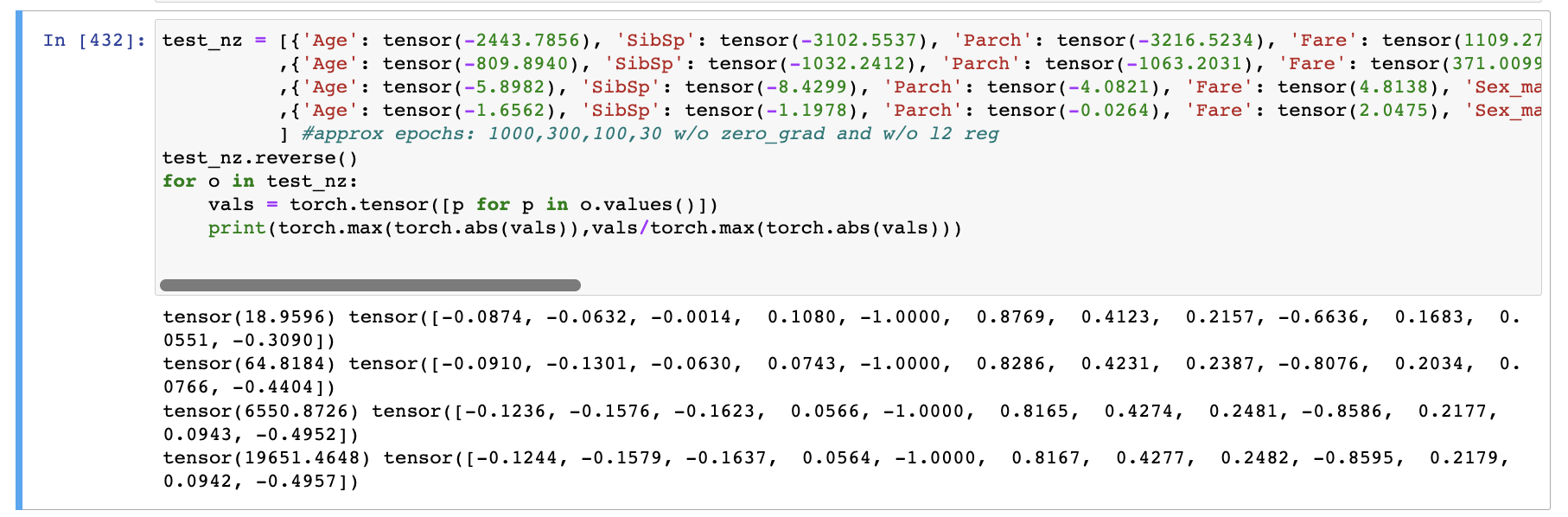
Finally, I recorded the coefficients across multiple runs with an increasing number of epochs, all without l2 reg. I observed that while the coefficients were continually growing, their relative values between one another was converging.

Code

trn_split, val_split = RandomSplitter(seed=SPLITTER_SEED)(t_indep)
len(trn_split), len(val_split)

trn_indeps, val_indeps, trn_deps, val_deps = t_indep[trn_split], t_indep[val_split], t_dep[trn_split], t_dep[val_split]

n_coeffs = t_indep.shape[1]
print('n_coeffs',n_coeffs)
def lin_init_coeffs():
    torch.manual_seed(TORCH_SEED)
    return (torch.rand(n_coeffs)-0.5).requires_grad_(True)
coeffs = lin_init_coeffs()

def lin_show_coeffs(coeffs): return dict(zip(indep_cols, coeffs.requires_grad_(False)))

def lin_update_coeffs(coeffs, lr=.01,zero_grad=True):
    with torch.no_grad():
        coeffs.sub_(coeffs.grad*lr)
        if zero_grad: coeffs.grad.zero_()

def lin_calc_preds(coeffs, indeps):
    return torch.sigmoid((indeps*coeffs).sum(axis=1))

def lin_calc_loss(preds, deps):
    return (preds - deps).abs().mean()

def lin_calc_acc(coeffs):
    with torch.no_grad():
        preds = lin_calc_preds(coeffs, val_indeps)
        ret = ((preds > 0.5) == val_deps.bool()).float().mean()
    return ret

def lin_calc_epoch(coeffs, indeps, deps, lr=2.,zero_grad=True,l2_reg=True):
    preds = lin_calc_preds(coeffs, indeps)
    loss = lin_calc_loss(preds, deps)
    if l2_reg: loss += (coeffs.square().sum()) * .001 #prevent unbounded growth of coeffs
#     print(f'loss {loss:.3f};',end='')
    loss.backward()
    grads = coeffs.grad.data.clone().detach().abs().mean()
    lin_update_coeffs(coeffs,lr,zero_grad=zero_grad)
    with torch.no_grad():
        val_preds = lin_calc_preds(coeffs, val_indeps)
        val_loss = lin_calc_loss(val_preds, val_deps)
    acc = lin_calc_acc(coeffs)
#     print(f'acc: {acc:.4f};',end='')
    return loss.detach(), val_loss.detach(), acc, grads, coeffs.clone().detach().abs().mean()

def lin_train_model(epochs=30, lr=2.,zero_grad=True,l2_reg=True):
    trn_loss,val_loss,acc, grads, coeffs_track = [],[],[],[],[]
    coeffs = lin_init_coeffs()
    for e in range(epochs):
        tl,vl,a,gr,c = lin_calc_epoch(coeffs,trn_indeps,trn_deps,lr,zero_grad=zero_grad,l2_reg=l2_reg)
        trn_loss.append(tl);val_loss.append(vl);acc.append(a);grads.append(gr);coeffs_track.append(c)
    print('\n',lin_show_coeffs(coeffs).__str__(),'\n')
    return trn_loss, val_loss, acc, grads, coeffs_track

def make_plot(tl,vl,acc,grads,coeffs_track,zero_grad,l2_reg):
    best_acc_epoch = np.argmax(acc)
    print(f'best acc epoch: {best_acc_epoch} | trn_loss: {tl[best_acc_epoch]} | val_loss: {vl[best_acc_epoch]} | acc: {acc[best_acc_epoch]}')
    print(f'last epoch: {len(acc)} | trn_loss: {tl[-1]} | val_loss: {vl[-1]} | acc: {acc[-1]}');xs = list(range(len(tl)))
    fig, (ax1,ax3) = plt.subplots(ncols=2,figsize=(16,6));ax2 = ax1.twinx();ax4 = ax3.twinx(); ax1.set_ylabel('Loss'); 
    ax2.set_ylabel('Accuracy');ax1.plot(xs,tl,label='tloss'); ax1.plot(xs,vl,label='vloss');ax4.plot(xs,coeffs_track,label='coeffs_abs_mean')
    ax2.plot(xs,acc,label='acc',color='g');ax3.plot(xs, grads, label='grads_abs_mean',color='red');fig.legend();
    ax3.set_ylabel('grads');ax4.set_ylabel('coeffs')
    title = f"{'With' if zero_grad else 'Without'} coeffs.grad.zero_() | "
    title += f"{'With' if l2_reg else 'Without'} coeffs l2 regularization (0.001)"
    _ = plt.title(title)

#EXAMPLE RUN:
make_plot(*lin_train_model(epochs=30, lr=2., zero_grad=(zero_grad:=False),l2_reg=(l2_reg:=False)),zero_grad,l2_reg)

Overall this was an interesting set of experiments and utilizing a simple linear model made it easier to wrap my head around everything that was going on. The graphs really helped visualizing what was going on during training.

Sorry for the super-long post!

EDITS:

  1. Added a reference to the course notebook I am referring to.
  2. Clarified question - Is omitting zeroing grads after epochs done on purpose or is it a bug.
  3. Clarified zero_grad is typically done at the end of one mini-batch/step, not epoch, but in this case since there is only one batch, a batch and epoch are the same thing.
  4. Jeremy confirmed gradients should be zeroed after each epoch in the referenced course notebook and it has been updated to add in that functionality so this question will no longer make sense if you view the notebook I was referring to. Here is a link to the version before it was added so you see what I was referring to originally: Linear model and neural net from scratch | Kaggle . It’s pretty cool that Kaggle keeps notebook revisions. Thank you Jeremy for the confirmation!
11 Likes

To get the weights zero centered i.e zero mean.

As I understand the gradients get accumulated. So they need to be zeroed after the weights are updated. Not sure why it does not matter here.

1 Like

It is normally done where during each training? and, it “seems like a bug” in what?

I must confess almost all of this is totally over my head. I guess I need to go back to that notebook and try to understand it better.

I have code in a python file which I import into Juypter. The initial import works as expected. The problem is that changes to the python file don’t appear to be reloaded after re-executing the cell with the import. In the past, the following magic Jupyter commands worked. Thanks in advance if anyone knows how to fix this.

%load_ext autoreload
%autoreload 2

Regarding tabular data. What is your experience with fastai? Is it on par with things like XGBoost or LightGBM? Or is it a similar case as with HF Transformers, where a third-party library is a better choice? Or would you advise starting with the fastai and migrate to something more specific later on? As far as I remember, boosted trees showed better results on tables compared to NNs. (Though I also remember things like TabNet.) Last time when I approached this question, gradient boosted ensembles showed better performance.

I’m curious if this was done on purpose, and if so for what reason, or if this is a bug. I am not sure why it’s not being done in the course notebook. I did edit my post to try and clarify.

Typically gradients are zeroed out after each training step/mini-batch by the optimizer. I’m trying to figure out if this omission in the course notebook was done on purpose, and if so - for what reason, or if this is a bug. I edited my post slightly to try and clarify my question.

Through my experiments, I found that the coefficients were growing linearly (forever) for each additional epoch and the gradients were not settling towards zero (when not zeroing grads). This is not ideal because the coefficients will eventually become too large and are also not settling in on any particular values (converging), though the magnitude of each individual coefficient with respect to each other does seem to converge. Also, the gradients are not settling towards zero, which they are normally expected to do when the model converges. I have not worked much with linear models or tabular data, but omitting zero_grad seems incorrect and the results seem sub-optimal given enough training epochs. If my intuition is wrong in this case or generally on this topic, I’m interested in knowing what I have wrong :slight_smile: I hope these posts sufficiently explain my thought process on the topic.

3 Likes

Okay thanks @matdmiller for explaining this, I learned something from it. I have read about “exploding gradients” in one of the previous DL courses I took, but I thought the frameworks took care of it. It seems in pytorch it has to be done explicitly by calling zero_grad() etc.

Based on what you explained, it appears zero_grad should be used, but maybe because it’s a toy example, it was omitted to not confuse the beginners? though I think it would be good to know this behaviour.

1 Like

I made an additional edit to my original post which I think is important after your comment. I originally said that the grads were usually zeroed after a training epoch, but they are actually typically zeroed out after a batch/mini-batch/step, not at the end of the epoch. In this specific case there is only a single batch per epoch, but my previous statement was confusing and not generally correct. I’m still curious why we’re not zeroing grads it though :slight_smile:

3 Likes

I hope Jeremy sees this and answers this :smiley:

2 Likes

Oops I forgot! :open_mouth:

Really great analysis @matdmiller :slight_smile: I better go fix the notebook!

3 Likes

This is a great analysis. You can probably see why the coeffs keep growing the way they do - the .grad attribute is growing bigger and bigger!

In fact, what I accidentally implemented there is an extreme version of something called momentum. We might have to look at that in the next lesson when we discuss my bug!..

9 Likes

Thanks for the clarification! This was my initial thought, but I have not done much work on training linear models or with tabular data so I wasn’t sure if there was a specific reason it should be omitted in these instances or not. After running the experiments, I became more convinced that it was likely a bug based on what was happening with the gradients and coefficients (weights).

I think this is a good example of how machine learning can be tricky to debug and how libraries like fast.ai are helpful for not only beginners, but also for experts in the field by automatically taking care of ‘boilerplate’ code for you and implementing best practices, reducing the chances of simple bugs and allowing you to focus on code specific to the problem you’re trying to solve. In this instance, no errors were thrown and the resulting accuracy was still good even with a simple but significant bug in gradient descent.

I feel like taking the time to not only understand the linear model course notebook, but re-writing the notebook (mostly) from scratch was helpful to reinforce many of the basic concepts that are required to train a model. I also think that having all of the code (except for data pre-processing) all together in one spot and nearly all fitting on to a single screen helps to demystify how each piece fits together. The linear model also has the benefit of nearly instantaneous training which allows for extremely fast iteration when trying out different things. I also found plotting the metrics particularly helpful to understand how the model was training and exactly what was going on internally.

Thanks! It’s interesting because you would expect the grads to start to diminish at some point even with the accidental extreme momentum, but because it seems the ratio of the coefficients is what the model converges on rather than specific values the grads eventually level off but coefficients keep growing with a relatively stable loss/accuracy.

3 Likes

Yes exactly - trying to write correct machine learning code is very hard, because errors often silently result in suboptimal results, rather than visible exceptions.

4 Likes