Interesting.
Have you tried “helping” SGD out, not starting from random inits but instead from more reasonable guesses?
Maybe it is just having hard times converging.
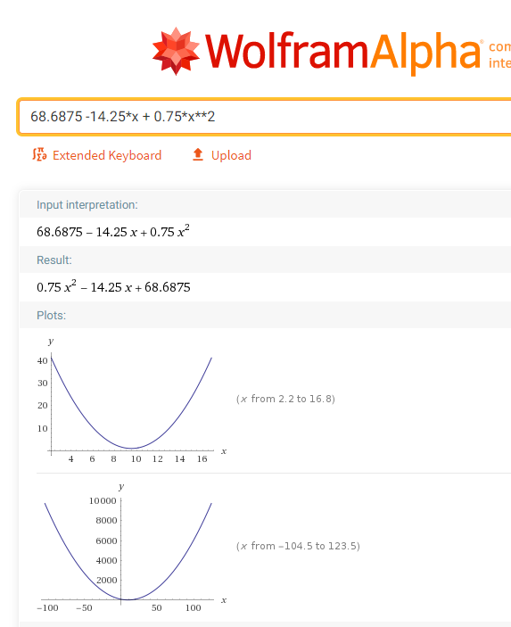
Your parabola is y = torch.randn(20)*3 + 0.75*(x-9.5)**2 + 1.
If we remove the torch.randn bit, that equals to y = a1(x-b1)**2 +c1 where
a1 = 0.75
b1 = -9.5
c1 = 1
Expanding and re-arranging gives (hopefully i did not screw up ) :
which means you are trying to fit the following parameters:
a1 = 0.75
2*a1*b1 = 2 * 0.75 * -9.5 = -14.25
c1 + a1*b1**2 = 1 + 0.75 * 9.5**2 = 68.6875
e.g. the curve at the bottom.
Thing is you are starting from these random values, which are quite distant from your final wanted output: tensor([0.1197, 0.5731, 0.7422], requires_grad=True)
My guess is that a more flexible optimizer such as Adam would be more appropriate, meaning that the same learning rate cannot possibly work for the 3 params at the same time.
Maybe worth initializing to something closer to the final result?
Thanks for posting an interesting question. It consumed my morning! But I certainly learned a lot from your code and various ML experiments.
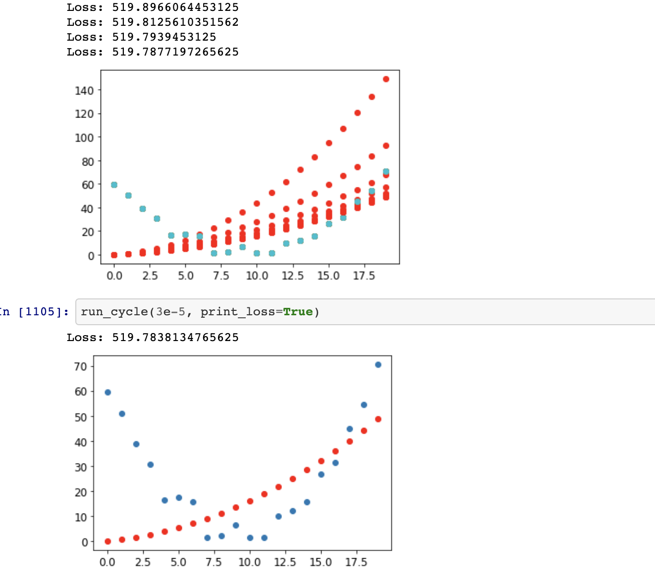
I think more than one issue explains what is happening. First, let’s eliminate the randomness from the y values. These can create local minima distant from the global minimum. Without an optimizer that uses some kind of momentum, the training can get stuck in one. I know this only because of experiments with conv1d and a piecewise linear toy problem.
But even without randomness, trying only to converge to an exact solution, training gets stuck far from the actual solution. It’s too slow with one lr and blows up (loss and gradients) with a higher lr. Here I think Francesco’s idea applies. You can see that one of the gradients quickly becomes 10x-100x larger than the others. When lr is small enough to handle the largest gradient, hardly any progress is made along the other dimensions.
Finally, if you take Francesco’s suggestion to initialize the params to near the actual solution, training still gets stuck at params near but not at the actual solution. Training converges, but would take days to reach the solution. Increasing the lr causes the loss blowup as above.
This is very similar to what I found with the above toy problem, and I’m guessing it’s the same idea. The loss landscape (in two parameters) was a valley with very steep sides following y=1-x. The valley floor sloped down to the exact solution but with an extremely small slope. The optimizer would jump from one side of the valley to the other making infinitesimal progress toward the solution. I was finally able to visualize this process with a 3-D plot.
So I think you have found a very instructive “pathological” case. No matter how the params are initialized, they drop down to some point along the valley. From there training makes negligible progress. You can’t increase the lr because one or more gradients are very sensitive to changes in the params. Happy hiking! May you arrive sometime next year.
I think an optimizer that works per parameter and with momentum may be worth trying. But FWIW, with my toy example ADAM also failed. I also speculate that such pathological examples are likely to be found in simple models with few parameters. More degrees of freedom may mean less chance of constructing such a “trap”.
Mostly speculation of course, but maybe it will help you to investigate further.
The problem is the true value for your function are much much larger than your initial conditions, so getting there with SGD is very slow.
Your function
y = torch.randn(20)*3 + 0.75*(x-9.5)**2 + 1
If you expand this out, you get
y = torch.randn(20)*3 + 0.75*x.pow(2) - 14.25*x + 68.68
It’s going to take a long time for a value year 0 to SGD to 68.68. I ran SGD for 600,000 iterations and got an error of 31. I also ran the optimization with Adam and got an error of 9.12 in 75,000 iterations.
Edit:
Also if you normalize your Y values to have a mean 0 and standard deviation of 1 you can get the same performance 30% of the iterations.
I got stuck with the same issue, and found that normalization fixes this and lets you converge to the ideal solution very quickly.
I have always learned to normalize the inputs, but never realized how dramatic the effects of not normalizing can be. I am surprised this wasn’t caught in the preparation for the course.
Perhaps because fast.ai focuses in image analysis, in which case all parameters are normalized by default (at least, they all have the same range).
 ) :
) :