Thanks.
Ha ha, I guess your smile looks like a tick!
Thanks.
Ha ha, I guess your smile looks like a tick!
Here is the question from the study group  :
:
When creating a new DataBlock using the batch_tfms , are the transformations applied at random to each batch as it is passed to our CNN?
And when using item_tfms arguments, the selected transform is only applied once to each item in the whole dataset, or does it get re-applied each epoch?
It gets re-applied each time you need to get that item. So it’s applied each epoch.
Depends on the transformation. Normalize will get applied equally to each batch, Rotation will get applied randomly.
Being a item_tfm or a batch_tfm does not define if the transformation will be random or not, you can have a random or deterministic item_tfm or batch_tfm
did you happen to get voila working in paperspace?
Im replacing notebooks with voila/render and get a 404
Finally got around to clean it up and push it to GitHub 
There even is a trick Jeremy describes to train your network using the same images, but on different sizes, as a form of data augmentation…
Pseudo steps:
data_224 (size 224)

create network with data_224

train network

save network ("some_name_224")

data_299 (size 299)

create network with data_299

load saved network "some_name_224"

train network
Hi darek.kleczek hope you are having a marvelous day!
I really enjoyed your notes, I thought they were a very clear summary.
We have similar hand writing so I found them easy to read.
Thanks for a great short and concise summary.
Cheers mrfabulous1
Thank you @mrfabulous1 - reading your comments on this forum always brings joy  Have a wonderful day/night depending what’s your time zone
You can also export your model to ONNX and deploy your model where you can use the ONNX runtime for serving the predictions. Please see this related post and the pointers to the code that is quite generic (though I wrote it for Azure Functions serverless deployment).
https://forums.fast.ai/t/exporting-a-model-for-local-inference-mode/66975/10?u=zenlytix
Gradient misunderstanding question!
Around 1 hour 50 seconds in the Lesson 3 part 1v4 video, Jeremy demonstrates getting the gradients, first for a float of 3.0, then for a tensor.
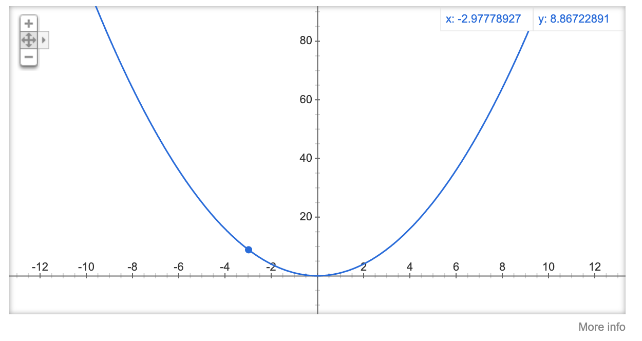
What I don’t understand (and this is definitely some elementary-level misunderstanding on my part) is that – just referencing the float for now – the gradient of 3.0 in the example is 6.0 (given the gradient of x^2 is 2x), but if we were to subtract the gradient (3.0-6.0) we’re left with -3.0, and this doesn’t feel very useful for anything.
What am I missing here?
The parameters in the model can be positive or negative  In reality our parameter update is typically never the full gradient, but a fraction of it. For example in the case below, where loss is on the y-axis, if we were to update the parameter (3.0) with the full gradient, we would end up at -3.0, like you said, which brings us no closer to the minimum loss
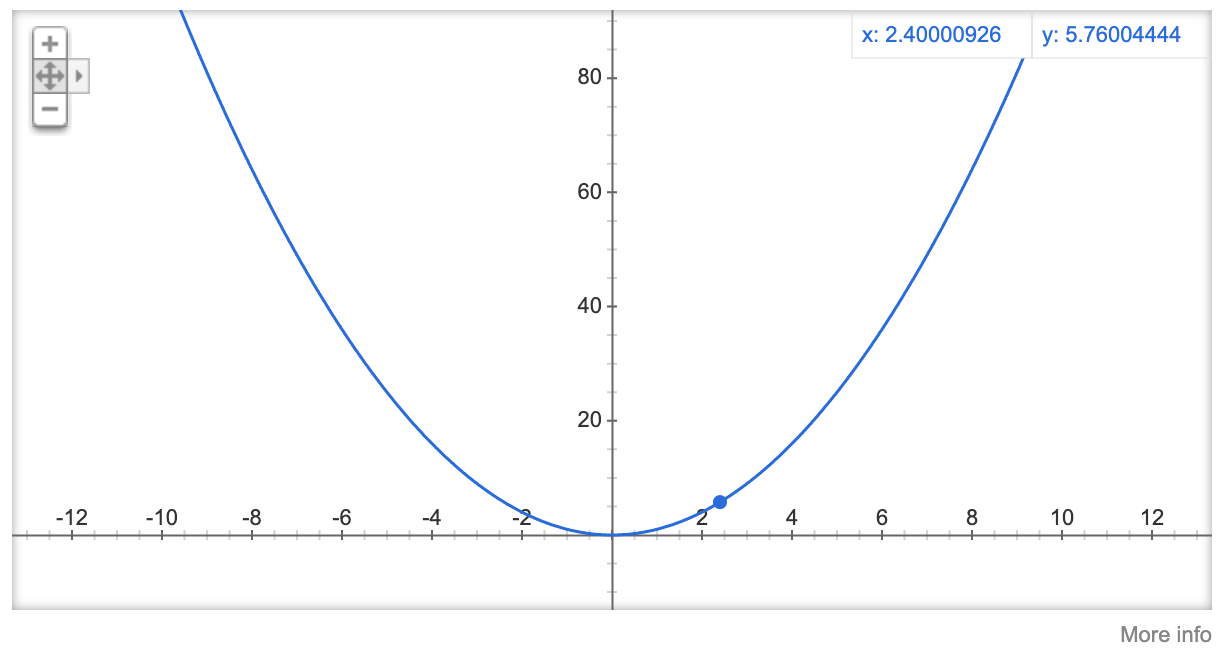
Instead we update the parameter with a fraction of the gradient, this fraction is the learning rate. If our learning rate is 0.1, then our paramter update will be 3.0 - (6.0 * 0.1) = 2.4, which brings us closer to the minimum loss:
I think thats the intuition behind it at least
@morgan Thanks for your response!
What I did’t understand (and I may well be answering my own question here, with this whole concept finally clicking) is:
Does this process only work with the addition of a learning rate?
ie, There is no scenario in which we can find the gradient and subtract it from our value in full, without ‘moderating’ it with a learning rate? Because if we did that, it would always cause an ‘overshoot’ of the minimum?
Interesting question! I hadn’t heard of it so I searched around and found Training Deep Networks without Learning Rates Through Coin Betting, which was presented at NeurIPS 2017, in which you don’t need a learning rate ![]() From the author’s Github:
From the author’s Github:
COntinuous COin Betting (COCOB) is a novel algorithm for stochastic subgradient descent (SGD) that does not require any learning rate setting. Contrary to previous methods, we do not adapt the learning rates, nor we make use of the assumed curvature of the objective function. Instead, we reduce the optimization process to a game of betting on a coin and obtain a learning rate free procedure for deep networks.
How do we reduce SGD to coin betting?
Betting on a coin works in this way: start with $1 and bet some money wt on the outcome of a coin toss gt , that can be +1 or -1. Similarly, in the optimization world, we want to minimize a 1D convex function f(w) , and the gradients gt that we can receive are only +1 and -1. Thus, we can treat the gradients gt as the outcomes of the coin toss, and the value of the parameter wt as the money bet in each round.
If we make a lot of money with the betting it means that we are very good at predicting the gradients, and in optimization terms it means that we converge quickly to the minimum of our function. More in details, the average of our bets will converge to the minimizer at a rate that depends on the dual of the growth rate of our money.Why using this reduction?
Because algorithms to bet on coins are already known, they are optimal, parameter-free, and very intuitive. So, in the reduction we get an optimal parameter-free algorithm, almost for free. Our paper extends a known betting strategy to a data-dependent one.Is this magical?
No, you could get the same results just running in parallel copies of SGD with different learning rates and then combining them with an algorithm on top. This would lead exactly to the same convergence rate we get with COCOB, but the advantage here is that you just need to run one algorithm!
And from a Pytorch forum post here:
Imagine running in parallel multiple optimization algorithms, each one with a different learning rate. Now, put on top of them a master algorithm able to decide which one is giving the best performance. This would give rise to a perfect optimization algorithm, at least for convex functions. And, indeed, this is exactly the MetaGrad algorithm from NIPS’16 (https://arxiv.org/abs/1604.08740 ).
Now, image instead having an infinite number of learners in parallel and the algorithm on top doing an expectation of all of them with respect to the best distribution of learning rates. The infinity makes things easier because now the update becomes in a simple closed form. And this is exactly how my algorithm works. The coin-betting trick is a just an easy way to design this kind of algorithms.
So yep, its possible! I wonder why it hasn’t been adopted…real world performance/implementation difficulties or just community momentum…
am I right that the same transforms, that have been randomly selected from batch_tfms for a batch, are applied to all items in the batch?! and that’s why they can be performed more efficiently on the GPU (same operations on all items)?
I reproduced lesson 3 on the full MNIST dataset. You can find it here:
Github repository:
Gist:
did you get an answer to this?
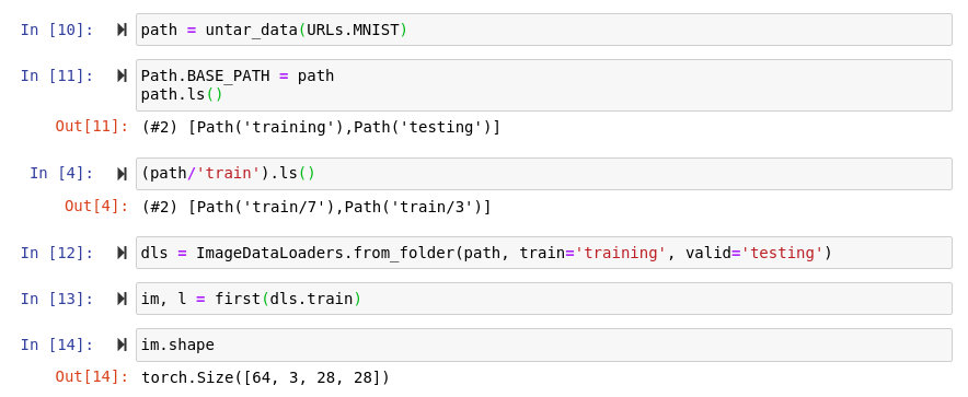
I’m loading the MNIST dataset with ImageDataLoaders.from_folder() and I’ve realised that the number of channels has been increased from 1 to 3 as shown below. Can anybody tell why it’s so. @muellerzr @radek
Probably because along with this we’re normalizing via imagenet_stats. Hence making it into a 3 channel image.
So if I get you correctly, ImageDataLoaders automatically normalizes every dataset with imagenet_stats right?
Actually I’m wrong, my apologies. The issue comes from the fact ImageDataloaders uses PILImage which opens it up in 3 channels, not PILImageBW which does 2. If you want that flexibility you should use the DataBlock API I believe here