i am struggling with this sentence in the Chapter 4 of the book:
Let’s check our accuracy. To decide if an output represents a 3 or a 7, we can just check whether it’s greater than 0.0, so our accuracy for each item can be calculated (using broadcasting, so no loops!) with:
i don’t understand why a positive prediction (preds>0.0) means a 3 and a negative prediction (preds<0.0) means a 7
it is not explained here
can somebody be so kind to explain or at least give me a hint
Yes I checked with notebook and video.
Listen to video 4 of 2020 version of the course Jeremy explained it between minute 14 to 18 . 2020 FASTAI
In short the reason is this : we choose anything bigger than 0 we call 3 and anything less than 0 we call 7. Then train our model based on this assumption. We can decide reverse and the model still works fine. (of course if we decide to do so Code need some changes ).
Then we make our prediction (negative and positive) to a float. (based on our training set format). If you look at it intuitively make sense too because it is either 3 or 7 so it is binary categorization.Since we label every 3 one and every 7 zero make sense to use positive for 3s and negatives for 7s
thank you, i feel like i am starting to get it ( ) but why 0 is the threshold? it feels arbitrary and enigmatic
also it seems the Course 2022 (which i am studying) differs significantly from Course 2020 but Course 2020 contains valuable hints and explanations which i miss from Course 2022
so is it worth to check those Course 2020 videos if i stuck somewhere? what do you think?
I studied 2022 version however some examples are based on the book that was published in 2020. it is possible to pick another threshold as long as it is one threshold for this problem. Like bigger than 1 or less than 1. Zero make sense more intuitively , everything less than zero become false and everything more than 0 will become True.For this specific chapter it is a good idea to listen to 2020 and 2022 version.
In this very basic model, the weights are initialized using torch.randn which produces a normal distribution of numbers, in this case with a mean of 0 and std of 1. So looking splitting the 2 classes at 0 makes sense because half of the weights should be > 0 and half should be < 0 so splitting at zero will give you approximately a 50/50 split. Later on in the chapter the sigmoid function is applied which produces results between 0-1 and then the prediction threshold is moved to 0.5.
The material is covered differently between the 2020 and 2022 courses so you will get value listening to/taking both courses.
Generally you want your numbers to stay close to 0 because due to how floating point numbers are implemented, the precision degrades the further away from 0 you get.
I think traditionally it comes from ‘logistic regression’ and the use of the ‘sigmoid function’ (if you want to dig a bit deeper you can have a look at those terms).
Most of the time you would not predict ‘high’ and ‘low’ values but (something that we interpret as) probabilities, so values between 0 and 1. The question the model then tries to answer is 'Is the given image a 3?" and the prediction 0.8 would mean that the model is 80% sure that the image is a 3.
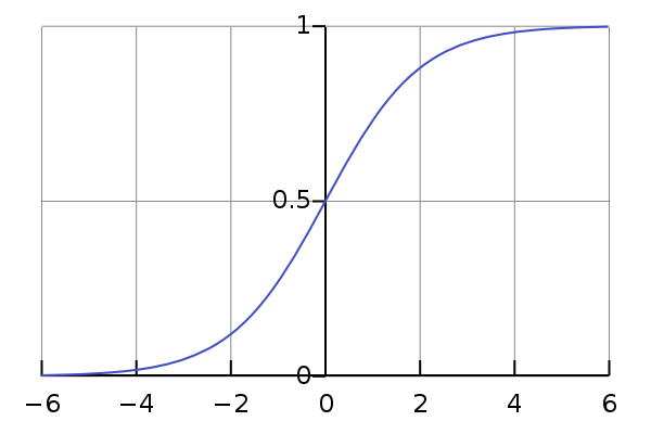
A way to get from arbitrary values to values in [0,1] is the sigmoid function which looks like this:
The larger the value you put into the function, the closer the result is to 1 and the ‘higher the probability’ that the image is a 3. Same for lower / close to 0 / not a 3, so a 7.
Now the threshold you would pick here most likely is 0.5. If the prediction is 0.49 that means 49% it’s a 3, 51% it’s a 7, so we obviously go with the 7. The twist is: which value do we need to put into the sigmoid function to land at 0.5? - Thats 0! So we can spare ourselves all that sigmoid business and just say: “values above 0 are label 3, lower than 0 are label 7”
Hope that makes sense
but why 0 is the threshold? it feels arbitrary and enigmatic
I was thinking about the same thing when working lesson 3 / chapter 4, tasking myself to implement a model for the full MNIST dataset. My take, as also mentioned in my notebook (section “Calculating the predictions (forward pass)”) is the following: Yes, you can simply make it up.
Why? For the task of predicting 3s and 7s, in the example, the model actually predicts values between 0 and 1, and that is what the model will converge to via gradient descent. You could have also picked 3 and 7 as output labels, and then determine if the predicted value is smaller/bigger than 5 to differentiate between 3s and 7s. The model would simply converge to different weights for calculating the values.
Similarly, when working on the full MNIST, I ended up picking just labels 0 to 9 by rounding the prediction results. What was striking me was that even with random weights, I had some correct predictions. And I guess the reason for that is that the possible space of output results was around the values 0 to 9. I think, this was more a coincidence because I had normalized all the pixels to values 0 to 1 (not 0 to 255). But I am quite sure that even without the normalization, the model would have converged. All the weights of the model simply would have to me multiplied by 255 - maybe that is oversimplifying, but something like that. Gradient descent will just do its magic.