Sometimes this paper implementation might be helpful for you.
1 Like
Ah yes, I read through his implementation. I think the main problem is that I wasn’t calculating the mask in the same latent space as the latents themselves, as @matdmiller mentioned here:
That is, my latents are 64x64x4 whereas I my mask is 512x512x3. So to apply the mask, I uncompressed my latents, applied the mask, and then recompressed the latents. Since the compression is lossy, I think that’s why the issue is occurring.
There are a few other differences from my implementation to the actual steps in the paper, but I don’t think they should make much of a difference.
I’ve decided to leave my implementation for now (have spent 2 weeks on it heh) and writing a post on my current implementation. Perhaps I’ll return to it later on in the course.
1 Like
I just figured out how exactly matrix multiplication works through broadcasting. That was an “Aha!” moment ![]() .
.
Here’s what’s happening.
Let’s say we have the following tensor of 2 images. Each row is a single image.
t1 = tensor([
    [1, 2, 3],
    [4, 5, 6],
])
Here is our tensor of 10 sets of weights. Each column is one set of weights.
t2 = tensor([
    [9, 6, 3],
    [8, 5, 2],
    [7, 4, 1]
])
t1.shape, t2.shape
(torch.Size([2, 3]), torch.Size([3, 3]))
Let’s get a single image.
t1[0].shape, t2.shape
(torch.Size([3]), torch.Size([3, 3]))
We can obviously do the dot product since the dimensions are compatible (t1 acts as a 1x3 tensor). However, this involves using at least 2 for loops, which is slow.
Instead, we can perform the dot product through elementwise multiplication and a single for loop. This is done through broadcasting. (More on the for loop part at the end of this post)
To do this, we need to transpose t1 so it’ll be a column vector/matrix.
t1[0, :, None].shape, t2.shape
(torch.Size([3, 1]), torch.Size([3, 3]))
Now the dimensions still aren’t compatible. However, we can broadcast t1 from this…
t1[0, :, None], t2
(tensor([[1],
         [2],
         [3]]),
 tensor([[9, 6, 3],
         [8, 5, 2],
         [7, 4, 1]]))
…to this.
t1[0, :, None].expand_as(t2), t2
(tensor([[1, 1, 1],
         [2, 2, 2],
         [3, 3, 3]]),
 tensor([[9, 6, 3],
         [8, 5, 2],
         [7, 4, 1]]))
Now we can perform elementwise multiplication.
t3 = t1[0, :, None] * t2; t3
tensor([[ 9,  6,  3],
        [16, 10,  4],
        [21, 12,  3]])
Each column in the resulting matrix is the result of multiplying the image with a particular set of weights (here, we’re multiplying a single image with 3 different sets of weights).
\begin{bmatrix} 1 & 1 & 1 \\ 2 & 2 & 2 \\ 3 & 3 & 3 \end{bmatrix} \odot \begin{bmatrix} 9 & 6 & 3 \\ 8 & 5 & 2 \\ 7 & 4 & 1 \end{bmatrix} = \begin{bmatrix} 1 \cdot 9 & 1 \cdot 6 & 1 \cdot 3 \\ 2 \cdot 8 & 2 \cdot 5 & 2 \cdot 2 \\ 3 \cdot 7 & 3 \cdot 4 & 3 \cdot 1 \end{bmatrix}
\odot denotes elementwise multiplication (also known as the Hadamard product; fun name heh).
To complete the dot product, we can simply sum each column.
t3.sum(dim=0)
tensor([46, 28, 10])
So the resulting dot product by applying the first image with the first set of weights is 46, with the second set of weights is 28, and the third set of weights is 10.
What about the for loop? Since we only applied the weights to a single image, we didn’t need a loop. However, if we have multiple images, we’ll need a single for loop to loop through each image/row in t1. If we didn’t use broadcasting, we’d have to use a for loop for looping through each image/row in t1 and another for loop for each set of weights/column in t2.
After writing this out, and if I’m not missing anything, I think it may be easier to make each row in t2 contain the weights, as opposed to the columns, as it would remove the need to transpose t1.
(Un)successfully finished my implementation of DiffEdit; you can read through it here.
While I managed to generate a mask…
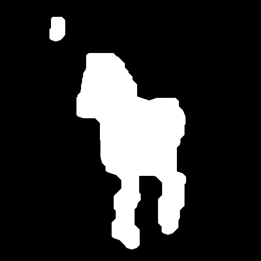
…I wasn’t able to apply it.
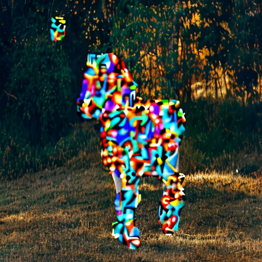
This is probably because I repeated uncompressed and recompressed the latents to apply the mask — VAE compression is lossy. My mask is 512x512x3 whereas my latent is 64x64x4.
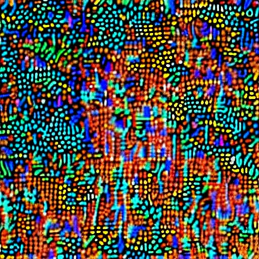
In fact, if I uncompress and immediately recompress a latent during each step in a normal stable diffusion implementation, this is the outcome.
Ended up using the Hugging Face Stable Diffusion Inpaint Pipeline.
Trying to implement DIffEdit.
For some reason, my original image is darker:

while my newly generated image is lighter. (Please see my reply, I have to split this into multiple replies due to forum’s constraint of 1 embedded media per new user.)
While my newly generated image is lighter:

This makes masking hard as I end up with something weird (one darker and the other lighter shade).
Has anyone faced this issue before?
I want to know a bit more on the DDIM process mentioned in the background section of DiffEdit paper. A quick google search returned a Keras implementation - Denoising Diffusion Implicit Models
Unfortunately I could not find any accessible PyTorch implementation with explanation. Would be grateful if the community could help with the same, thanks in advance!
We cover it in this course.
1 Like
Hi,
Does anyone know what does Jeremy uses to effortlessly (or at least the effort is not visible on the video) to draw on onenote or on Jupyter notebooks? Those drawings immensely helped me to understand broadcasting
Thanks
I use a graphics tablet. Onenote lets you draw directly. For other apps like Jupyter I use this: https://presentify.compzets.com/
1 Like
Thanks for sharing the details
Made a quick implementation of DiffEdit in a notebook using the Stable Diffusion Deep Dive notebook as a base. Any feedback is welcome!
In case helpful to anyone else new to the math as well, I wanted to share that that ChatGPT 4 is pretty effective here. You can take a screenshot of the equation, ask it to be explained to you, and get fairly detailed responses – even without providing it any additional context from the paper:
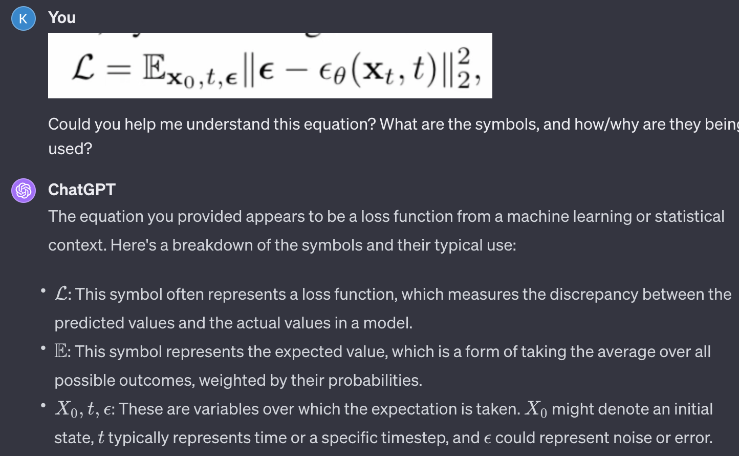
1 Like
I just watched the part of the lecture where JH implements fast matrix multiplication from scratch using broadcasting.
He does this by iterating over each row in the first matrix and broadcasting that row to the second matrix. I assume this is faster because the broadcasting operations all happen in parallel.
The previous inferior version he implemented used iteration over both dimensions and so nothing happened in parallel. But then he replaced one of the iterations with a broadcast, speeding it up.
My question is: why not take this a step further and replace the remaining iteration with broadcasting as well?
Then all the rows of the first matrix could be broadcast to the second broadcast step in parallel. Wouldn’t that speed it up even more?
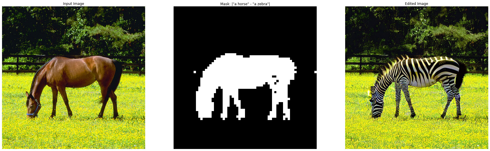
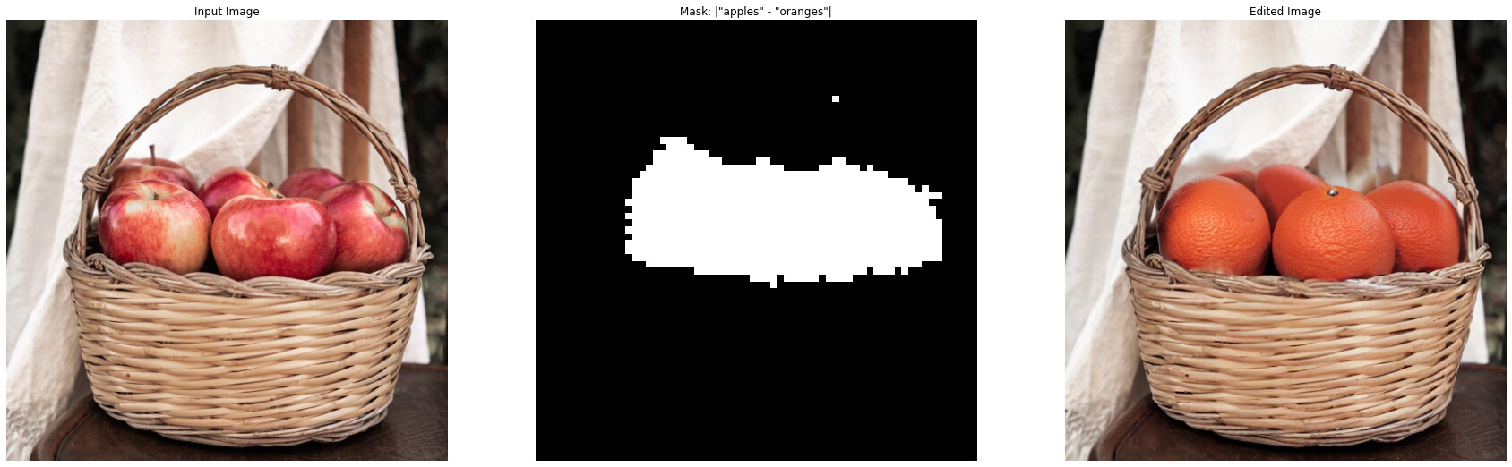
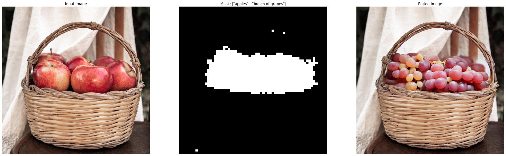
I know I am late to the party on DiffEdit implementation, but here is my take and results on it if anyone is interested in 2024:
Notebook
20240405_diffedit_consolidated.ipynb
Summary
- I used LMSDiscreteScheduler just like in lesson 9 nb.
- I removed extreme values in noise prediction difference by clipping bottom and top 10% values. This is a hyper-parameter that can be changed, but the default value of 10% works well. This step is also mentioned in the paper in Section 3.2 Step1.
- I averaged the noise difference over 10 random runs. This is also mentioned in the paper in Section 3.2 Step 1. Combination of step 2 and 3 gives high quality and stable masks.
- Image generation given mask is very similar to Image2Image example discussed in lesson 9. With slight modification towards the end of the loop where mask is used to replace background latent pixels with corresponding latent pixels from the forward diffusion process.
Results
4 Likes
I worked on implementing diffedit, it’s still not as good as i’d like it to be but here is the code if anyone is interested: GitHub - karthikven/DiffEdit
Hi,
I am working through the Broadcasting rules of lesson 11.
I am puzzled about matrix multiplication commutativity.
c[None,:] * c[:,None] is a multiplication between a 3:1 matrix and a 1:3 matrix, so I expect the dimension of the result to be 3:3, as is computer by JN.
However, if I invert the terms of the multiplication, I would expect a 1:3 matrix times a 3:1 matrix gives a 1:1 (a scalar = 1400), but I get the same 3:3 result.
That’s strange, no ?
PS: If a is a 3:1 matrix and b a 1:3 matrix, matmul(a,b) and matmul(b,a) works as expected (matmul(a * b) is a 3:3 matrix and matmul(b * a) is a 1:1 matrix)
1 Like
Puzzled me as well but it turns out element-wise multiplication in programming (such as with * in many libraries like NumPy or APL) is not the same as the matrix multiplication defined in traditional mathematics (like the dot product or inner product )
Element-wise Multiplication (*) or Hadamard product
multiplies corresponding elements of two arrays or matrices. Each element in one matrix is multiplied by the corresponding element in the other matrix.
Matrix Multiplication (Dot Product)
When multiplying two matrices, the number of columns of the first matrix must match the number of rows of the second matrix . The result is a new matrix, where each element is the dot product of corresponding rows and columns.
@Pierrot . It puzzled me as well but it turns out element-wise multiplication in programming (such as with * in many libraries like NumPy or APL) is not the same as the matrix multiplication defined in traditional mathematics (like the dot product or inner product )
Element-wise Multiplication (*) or Hadamard product
multiplies corresponding elements of two arrays or matrices. Each element in one matrix is multiplied by the corresponding element in the other matrix.
Matrix Multiplication (Dot Product)
When multiplying two matrices, the number of columns of the first matrix must match the number of rows of the second matrix . The result is a new matrix, where each element is the dot product of corresponding rows and columns.