Here is my understanding maybe that helps (if I am wrong someone correct me):


For more details one can look at the step function via
??scheduler.step
Here is my understanding maybe that helps (if I am wrong someone correct me):
Ah, I finally get scheduler.step! I was getting confused because for some reason, I was thinking that the unet also removes noise. But no, it’s the scheduler that’s removing the noise through the step method.
I’m still a bit confused over latents = latents * scheduler.init_noise_sigma and inp = scheduler.scale_model_input though.
Judging from what I’m reading in the screenshots, I think the first line scales the noise to a certain distribution, and the second line further scales the noise to match the K-LMS algorithm.
So is the first line preparing a foundation of sorts from which noise can be further scaled to match whatever algorithm we wish?
But that brings up another question: if my understanding above is correct, the scheduler object we have was instantiated from a class that is for the K-LMS algorithm. So why does the noise have to be scaled twice?
scheduler = LMSDiscreteScheduler(...)
No the unets task (as far as i understand is) to predict the noise residuals.
Today and tomorrow i am very busy at work.
I will try to look into more detail at friday or saturday and write more detailed explanantion.
But what we can directly see: at beginning we can almost neglect the +1 in the square root. So we rescale to unit variance.
Yeah, the U-Net predicts the noise in the image, which is then subtracted by the scheduler.
Sure! Explain when you have the time. ![]()
Yes, removing the 1 does approximate it to a distribution of N~(0, 1). ![]()
for i, t in enumerate(tqdm(sched.timesteps)):
  # For CFG
  inp = torch.cat([lats] * 2)
  inp = sched.scale_model_input(inp, t)

  # Predict noise residual.
  with torch.no_grad(): pred = unet(inp, t, encoder_hidden_states=txt_embs).sample

  # Perform guidance.
  pred_uncond, pred_txt = pred.chunk(2)
  pred = pred_uncond + g_scale * (pred_txt - pred_uncond)

  # Compute the "previous" noisy sample.
  #  Not quite sure what's happening here.
  lats = sched.step(pred, t, lats).prev_sample
Let’s explain line by line.
lats = lats * sched.init_noise_sigma
this does inital scaling to N(0,\sigma_T), where \sigma_T is the variance for the last timestep our schedule (we start with T, then T-1, …, then finally 1).
Note that \sigma_1>\sigma_0 etc. We gradually tune down the noise in our schedule.
Then we loop over the scheduler timesteps.
Note: As mentioned above we start from the last timestep (with largest noise) and then go down one timestep for each iteration.
inp = torch.cat([lats] * 2)
simply copies the latent vector into two samples. Why? Because we have also two prompts in our text embedding. The unconditional empty string embedding and our prompt.
Next step:
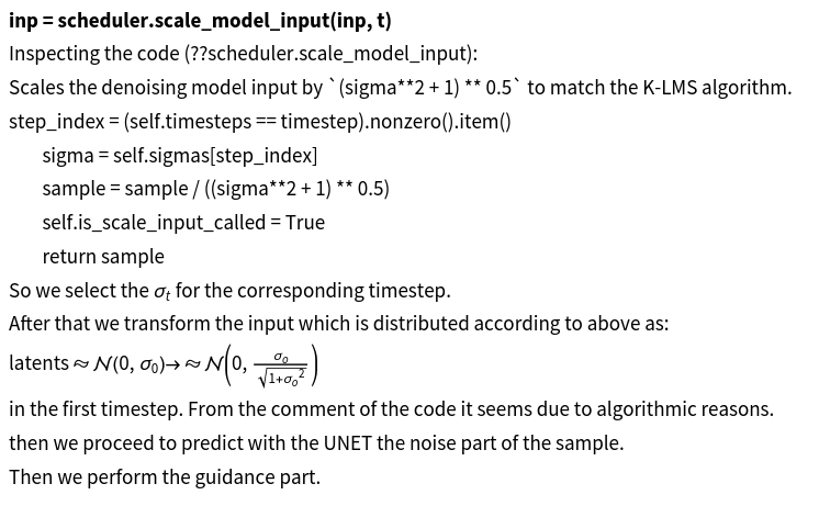
inp = sched.scale_model_input(inp, t)
according to the documentation of the scheduler this step is only needed for algorithmic purpose. In the doc we find:
    def scale_model_input(
        self, sample: torch.FloatTensor, timestep: Union[float, torch.FloatTensor]
    ) -> torch.FloatTensor:
        """
        Scales the denoising model input by `(sigma**2 + 1) ** 0.5` to match the K-LMS algorithm.
        Args:
            sample (`torch.FloatTensor`): input sample
            timestep (`float` or `torch.FloatTensor`): the current timestep in the diffusion chain
        Returns:
            `torch.FloatTensor`: scaled input sample
        """
        if isinstance(timestep, torch.Tensor):
            timestep = timestep.to(self.timesteps.device)
        step_index = (self.timesteps == timestep).nonzero().item()
        sigma = self.sigmas[step_index]
        sample = sample / ((sigma**2 + 1) ** 0.5)
        self.is_scale_input_called = True
        return sample
So this just grabs \sigma_t and rescales the variance of the input to make the algorithm work.
Next step is the unet, which just predicts the noise residuals. Then we perform guidance.
The larger we set the guidance constant g_{scale} the more we bias towards the original prompt.
Then we use the step function of the scheduler:
This is the code:
    def step(
        self,
        model_output: torch.FloatTensor,
        timestep: Union[float, torch.FloatTensor],
        sample: torch.FloatTensor,
        order: int = 4,
        return_dict: bool = True,
    ) -> Union[LMSDiscreteSchedulerOutput, Tuple]:
        """
        Predict the sample at the previous timestep by reversing the SDE. Core function to propagate the diffusion
        process from the learned model outputs (most often the predicted noise).
        Args:
            model_output (`torch.FloatTensor`): direct output from learned diffusion model.
            timestep (`float`): current timestep in the diffusion chain.
            sample (`torch.FloatTensor`):
                current instance of sample being created by diffusion process.
            order: coefficient for multi-step inference.
            return_dict (`bool`): option for returning tuple rather than LMSDiscreteSchedulerOutput class
        Returns:
            [`~schedulers.scheduling_utils.LMSDiscreteSchedulerOutput`] or `tuple`:
            [`~schedulers.scheduling_utils.LMSDiscreteSchedulerOutput`] if `return_dict` is True, otherwise a `tuple`.
            When returning a tuple, the first element is the sample tensor.
        """
        if not self.is_scale_input_called:
            warnings.warn(
                "The `scale_model_input` function should be called before `step` to ensure correct denoising. "
                "See `StableDiffusionPipeline` for a usage example."
            )

        if isinstance(timestep, torch.Tensor):
            timestep = timestep.to(self.timesteps.device)
        step_index = (self.timesteps == timestep).nonzero().item()
        sigma = self.sigmas[step_index]

        # 1. compute predicted original sample (x_0) from sigma-scaled predicted noise
        if self.config.prediction_type == "epsilon":
            pred_original_sample = sample - sigma * model_output
        elif self.config.prediction_type == "v_prediction":
            # * c_out + input * c_skip
            pred_original_sample = model_output * (-sigma / (sigma**2 + 1) ** 0.5) + (sample / (sigma**2 + 1))
        elif self.config.prediction_type == "sample":
            pred_original_sample = model_output
        else:
            raise ValueError(
                f"prediction_type given as {self.config.prediction_type} must be one of `epsilon`, or `v_prediction`"
            )

        # 2. Convert to an ODE derivative
        derivative = (sample - pred_original_sample) / sigma
        self.derivatives.append(derivative)
        if len(self.derivatives) > order:
            self.derivatives.pop(0)

        # 3. Compute linear multistep coefficients
        order = min(step_index + 1, order)
        lms_coeffs = [self.get_lms_coefficient(order, step_index, curr_order) for curr_order in range(order)]

        # 4. Compute previous sample based on the derivatives path
        prev_sample = sample + sum(
            coeff * derivative for coeff, derivative in zip(lms_coeffs, reversed(self.derivatives))
        )

        if not return_dict:
            return (prev_sample,)

        return LMSDiscreteSchedulerOutput(prev_sample=prev_sample, pred_original_sample=pred_original_sample)
I think what we do here is simply that we take our latents, our predicted noise for current timestep and the current amount of noise.
Then we return what we believe to be the latent at timestep t-1.
The returned sample should have variance \sigma_{t-1}.
From the code above its also clear how we use our predicted noise:
derivative = (sample - pred_{original.sample}) / \sigma
We take our sample, substract the noise and rescale the resulting sample in variance. (Note that if we predicted the noise perfectly then sample - pred_{original.sample} would be a fully denoised picture.)
Then we use this to make a step into the right direction (Jeremy explained this in more detail in lecture 9 i think and made analogy to the usual learning process in DL).
Then we reiterate this process until we reach the last timestep where the returned sample should have variance \sigma=0.
If we decode this, it will give us a non noisy, ordinary picture.
I hope this made things more clear.
Essentially what we try to do is the following:
Assume someone took a picture and blurred it up more and more at every timestep. How can we learn to reverse this process. As a guidance for what the picture should contain (and not contain) we have our prompt and potentially negative prompt instead of uncond_text, as well as the blurry (or at the end less and non blurry picture). We predict the noise in the picture and use this information to denoise the picture gradually with each timestep.
I appreciate the detailed explanation! This helped clear things up.
One thing that’s not yet quite making sense to me though is why we calculate the latent at the previous timestep.
lats = sched.step(pred, t, lats).prev_sample
The latent has already been denoised with the following line.
pred = pred_uncond + g_scale * (pred_txt - pred_uncond)
So can’t we simply let lats = pred for the next loop?
Note that the PREVIOUS STEP in time is the NEXT STEP in our loop ;-).
We progress backwards in time.
Also if you would set lats = pred that would not make sense: pred is linear combination of stuff we get from the unet and unet predicts noise. we want to get original image.
we use the predictions to denoise our latents gradually! they are not prediction of the timestep before.
Ahh, I think I get it now! The step number goes down in each proceeding iteration. Subtle detail heh.
Also if you would set lats = pred that would not make sense: pred is linear combination of stuff we get from the unet and unet predicts noise. we want to get original image.
Yeah, that makes sense. I was jumbling up the process in my mind.
pred = pred_uncond + g_scale * (pred_txt - pred_uncond)
pred_uncond is the unconditional noise, while pred_txt is the prompt noise. I was thinking one of them was the latent for some reason.
Thank you for your help!
After doing this lesson, I managed to implement my own custom stable diffusion class using the Diffusers library, and that was pretty satisfying heh.
I also managed to implement callbacks and negative prompts too!
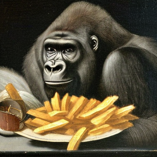
Prompt = ‘An antique 18th century painting of a gorilla eating a plate of chips.’
Negative Prompt = ‘plate’
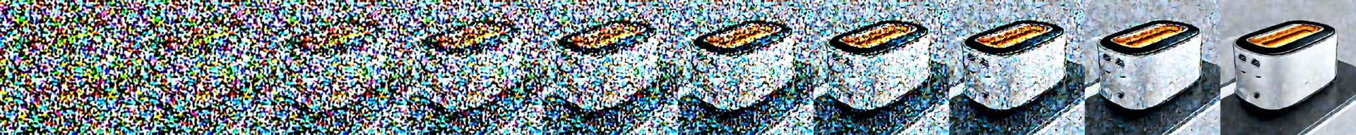
Prompt = ‘A toaster in the style of Jony Ive; modern; realistic; different; apple; form over function’
However, I didn’t quite manage to get image to image working htough.
I’ve written up how I implemented my own class in the blog post below.
After learning about how progressive distillation works, I can’t help but wonder if I’ve thought of a way to improve it:
Rather than having a single student approximate all the steps of the teacher’s denoising at once, why not have each round of progressive distillation involve twice the number of student UNets? This way, each student could specialize in a single pair of stages of denoising, which would be quite different tasks depending on how early or late in the process those stages are. I hypothesize that this would improve the quality of inferences, which in turn would make it possible to reduce the number of diffusion stages in the final distilled system.
Downsides of this would include 1) much more space/RAM required for the finished distilled model, which would actually be several models stapled together, and 2) no flexibility in terms of the number of denoising stages you want to use when the model is deployed. So there are big tradeoffs, but you could get the performance boost of distillation with higher-quality results (or better performance with identical-quality results, or somewhere in between those two).
Am I making sense?
I’m having trouble getting the stable diffusion notebook to run locally. I have pip3 installed diffusers and transformers. However, I get the following errors (which I can’t find references to in Google search):
File ~\AppData\Local\Programs\Python\Python312\Lib\site-packages\diffusers\pipelines_init_.py:47
45 from …utils.dummy_torch_and_transformers_objects import * # noqa F403
46 else:
—> 47 from .alt_diffusion import AltDiffusionImg2ImgPipeline, AltDiffusionPipeline
48 from .audioldm import AudioLDMPipeline
49 from .controlnet import (
50 StableDiffusionControlNetImg2ImgPipeline,
51 StableDiffusionControlNetInpaintPipeline,
52 StableDiffusionControlNetPipeline,
53 )
File ~\AppData\Local\Programs\Python\Python312\Lib\site-packages\diffusers\pipelines\alt_diffusion_init_.py:31
27 nsfw_content_detected: Optional[List[bool]]
30 if is_transformers_available() and is_torch_available():
—> 31 from .modeling_roberta_series import RobertaSeriesModelWithTransformation
32 from .pipeline_alt_diffusion import AltDiffusionPipeline
33 from .pipeline_alt_diffusion_img2img import AltDiffusionImg2ImgPipeline
File ~\AppData\Local\Programs\Python\Python312\Lib\site-packages\diffusers\pipelines\alt_diffusion\modeling_roberta_series.py:6
4 import torch
5 from torch import nn
----> 6 from transformers import RobertaPreTrainedModel, XLMRobertaConfig, XLMRobertaModel
7 from transformers.utils import ModelOutput
10 @dataclass
11 class TransformationModelOutput(ModelOutput):
ImportError: cannot import name ‘RobertaPreTrainedModel’ from ‘transformers’ (C:\Users<user>\AppData\Local\Programs\Python\Python312\Lib\site-packages\transformers_init_.py)
Any ideas?
I found generators a bit tricky to understand properly, so I’ve put together a list of 10 practice questions to help practice generators in python. You can find both the questions and solutions here: fastai-p2/generators_practice_questions.txt at main · karthikven/fastai-p2 · GitHub.