Thank you - I will try to bring in dataloader counts and see how this makes a difference!
Since ‘register_forward_hooks’ function can modify the output, can we implement BatchNorm using pytorch hooks ? I’ll try it and see what happens
Trying this again after a small break due to work reasons…
I tried running your statement @akashpalrecha and it returns 97 and not 108 for train_dl. I presume you meant train and valid combined, which gives the correct number. Thanks again for the tip!
Giving my thoughts here for future readers stuck on a similar issue. We have 50,000 images in train_dl with a batch size of 512 so 97.6 (98) iterations are needed to cover all the train_dl images.
For valid_dl, we have 10,000 images but a batch size of 1024 (as batch size is doubled for validation). This results in 9.7 (10) iterations needed to cover valid_dl images.
So a total of 108 iterations are needed in 1 epoch, which explains 216 for 2 epochs!
Good thought… please share your findings… look forward to it.
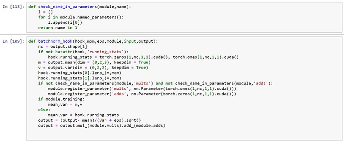
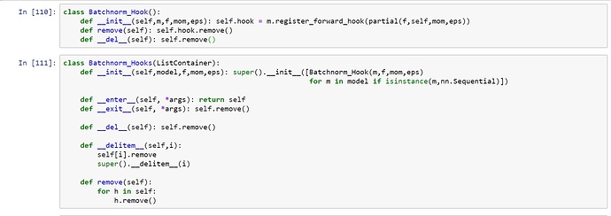
I was curios if we can implement batchnormalization using pytorch hooks, since 'register_forward_hook" can modify output of a module. So I went ahead and implemented batchnorm using hooks. It’s lot less flexible and not a recommended thing to do but I did it just for the sake of it 
-
Defining the callback function that ‘register_forward_hook’ will call:-
-
Modifying the Hook and Hooks classes:
3.Running the model using these hooks on mnist data:
The performance isn’t at par with normal nn.Batchnorm layer. What could be the reason behind that?
Lesson 10. 1:14:10
Why the mean and std of the layer outputs (not weights) show us if the training going well or not?
My notes on this lesson: https://jimypbr.github.io/2020/03/fast-ai-lesson-10-notes-looking-inside-the-model
Hello guys, I have a question about BatchNorm. I don’t know if this was asked before but i couldn’t find it.
So this was the BatchNorm class implemented on the lesson:
>>class BatchNorm(nn.Module):
    def __init__(self, nf, mom=0.1, eps=1e-5):
        super().__init__()
        # NB: pytorch bn mom is opposite of what you'd expect
        self.mom,self.eps = mom,eps
        self.mults = nn.Parameter(torch.ones (nf,1,1))
        self.adds  = nn.Parameter(torch.zeros(nf,1,1))
        self.register_buffer('vars',  torch.ones(1,nf,1,1))
        self.register_buffer('means', torch.zeros(1,nf,1,1))

    def update_stats(self, x):
        m = x.mean((0,2,3), keepdim=True)
        v = x.var ((0,2,3), keepdim=True)
        self.means.lerp_(m, self.mom)
        self.vars.lerp_ (v, self.mom)
        return m,v

    def forward(self, x):
        if self.training:
            with torch.no_grad(): m,v = self.update_stats(x)
        else: m,v = self.means,self.vars
        x = (x-m) / (v+self.eps).sqrt()
        return x*self.mults + self.adds
Now, I think I understood the normalization part(linear interpolation etc.).
But the part that I didn’t understand is; how we use self.mults and self.adds(gamma and beta). And in paper they are described as: “Parameters to be learned.”
They are not effective with their initial values. And we are not updating them either(in here or later in training). How are they useful. Am I missing something here?
I’m going to answer as my understanding, so it might be wrong:
In that graph, we have 6 different plot for every layer. So if we inspect one plot(line), we see how means are doing from mini-batch to mini-batch for one layer. And since we are using stochastic gradient descent(which means gradient descent on minibatches), we are seeing how our activations are updated from mini-batch to mini-batch. When gradient grows too big, it causes to falling cliffs. Which is not a good thing. It causes to loose information and some of our acitivations are being nearly zero after this processes.
So it effects training. To prevent this kind of situation we will use initialization methods i think.
mults and adds are declared as nn.Parameter objects in the constructor. This registers them as being in a list of learnable parameters in that layer. They are then updated in the optimization step:
with torch.no_grad():
    for p in model.parameters(): p -= p.grad * lr
    model.zero_grad()
In other words, by declaring them as a nn.Parameter they will appear in the model.parameters(). Their grads are calculated by PyTorch.
Hi all!
So I am in lesson 10 at time 1:16, when Jeremy is explaining why the model layer mean activations are going up exponentially then crashing. So as he explains, as the mean activations are quite low already at layer 1, so at each subsequent layer the activations get exponentially smaller. So in the last layer they are tiny, so when we start propagating the gradients backwards they are going to be very small, especially by the time they get to the first layers.
So this all makes sense to me. It’s the next bit Jeremy says that I’m finding a little hard to understand, when he says:
“…so gradually it was moving into spaces that had some gradient, but by the time it got there the gradient was so fast that it was falling off a cliff and was having to start again.”
I can see the first part of this, so yes its gradually moving into spaces that have some gradient… its more the next bit… ‘by the time it got there the gradient is going so fast its falling off a cliff…’ etc etc. So to me because of the gradients should be getting smaller and smaller, this would have I thought caused the gradients to get smaller and smaller i.e so this should update the parameters less and less. So while initially the tiny gradients moved it a little the right way, because they vanish - you end up with it not going the right way more and more, or the model becoming more static i.e. with parameters hardly changing?
So if anything - I would have expected the mean activations to taper off like a log function and become a straight line? I don’t understand what is driving the mean activations to explode exponentially then crash - given the gradients are tending to zero?
Would appreciate any helping in understanding this! thanks.


