I read the paper and this lesson notes but something was missing. I hope this is right and if so it can help others to fill the gaps I had myself regarding this lesson.
With Naive Bayes we obtain probabilities [0…1]
Prob(class=1|document) = P(1|d)
or
Prob(class=0|document) = P(0|d)
If we divide them, we have
y = P(1|d) / P(0|d) with values [0…inf] * being
y>1 → class=1
y<1 → class=0
- It will never be inf because we will add something later
that will make P(0|d) > 0
That’s all for operations on the left side of the equation.
On the right side we have
P(1|d) = P(d|1)*P(c=1) / P(d)
and
P(0|d) = P(d|0)*P(c=0) / P(d)
Dividing them
y = P(1|d) / P(0|d)
y = P(d|1)*P(c=1) / P(d|0)*P(c=0)
being
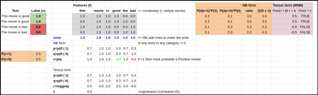
P(d|1)= product(fi * P(fi|1)) = ∏ (fi * P(fi|1))
P(d|0)= product(fi * P(fi|0)) = ∏ (fi * P(fi|0))
The ∏ is across all the fi contained in d (doc=d)
However the P(fi|1) and P(fi|0) are across all documents (D) (vertically)
and
P(c=1)= sum(cases with c=1) / N_cases_c=1
P(c=0)= sum(cases with c=0) / N_cases_c=0 = 1-P(c=1)
The trick mentioned before is that we will introduce 2 rows in our data matrix D

c=0  f=[1,1,1,......]
c=1  f=[1,1,1,......]
Dividing them
P(1|d) / P(0|d) = ∏ ( (P(d|1)/P(d|0)) * (P(c=1) / P(c=0)) )
If we define
pi = P(fi|1) = ∑ (fi when c=1) / N_c=1 (across all documents)
qi = P(fi|0) = ∑ (fi when c=0) / N_c=0 (across all documents)
P(d|1) = ∏ fi * P(fi|1) = ∏ fi * pi
P(d|0) = ∏ fi * P(fi|0) = ∏ fi * qi
then
P(1|d) / P(0|d) = ∏ ( (pi/qi) * (P(c=1) / P(c=0)) )
Now we take logs
log(P(1|d) / P(0|d)) =
= log (∏ ( (pi/qi) * (P(c=1) / P(c=0)) ) )
= log (∏ ( (pi/qi) + log(P(c=1) / P(c=0))
= ∑ log(pi/qi) + log(P(c=1) / P(c=0))
= ∑ ri + b
for i in elements of d (for ∏ and ∑)
Which seems very much like
pre_prediction = wi @ ri + b
being:
- wi the fi elements in d
- ri across all documents
- @ is matrix multiplication
- b is an escalar
because pre_prediction is a log(P(1|d) / P(0|d))
if pre_prediction >0 → prediction=1
otherwise → prediction=0
So we have transformed
- probabilities into a ratio of probabilities (and then taken the logs)
- a product (∏) into a summation (∑) by taking the logs
- Naive Bayes equations into something very similar to Logistic Regression
I also created a public sheet (I was missing it on the course material) in order to calculate and play with all the stuff myself.
You can copy it & play from here
Corrections and additions are welcome.
Issue:
We have
pre_prediction = wi @ ri + b
pre_prediction = log(P(1|d) / P(0|d)) = ∑ ri + b
BUT, that is true ONLY if the fi elements in
d = [ f1, f2, f3, …]
are binary, that is, either 1 or 0.
That may/would explain why using the binary form of the features matrix produces slightly better results. I’d say, it is not better, the problem is that wi @ ri + b is not fully correct and therefore produces worse results.
I hope someone could explain this difference.