Less accuracy on Music Genre classifier

I’m trying to implement a Music Genre Classifier using CNNs, wherein I first convert music file into a spectrogram( Image for representing audio in frequency vs time graph) and then pass into the CNN model to classify it.
I first created the spectrograms of the music files in GTZAN dataset which contains 100 examples for 10 genres, using a python script.
I tried both fastai library and keras for this model, but the not even getting accuracy >35%

I have already generated the spectrograms of the GTZAN dataset’s music file through a python script. Here’s the link to the dataset of the spectrogram

1) With RGB Images
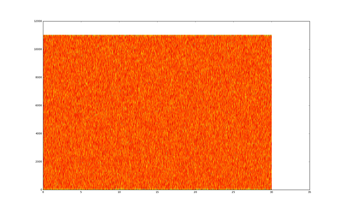
This is a spectrogram represeting a music file of rock genre


I distributed those images in same fashion, like in the cats v dogs wherein I created train,test,valid and sample folder. Then I ran the classifier of lesson 1 using resnet34 architecture, but I’m getting very less accuracy, about (14-35%) and the accuracy changes a lot even if I run the same cell again. Here’s the iPython Notebook and the data used for this notebook.

2) With Grayscale Images
Then my friend suggested me, to convert those RGB spectrogram into grayscale spectrograms. I tried that, but didn’t work, I was getting the accuracy around 23% even after using the best learning rate from the learning rate finder.
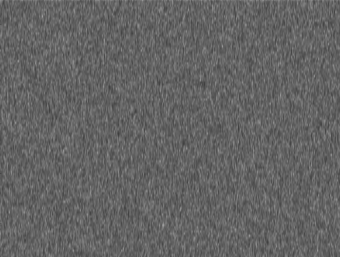
This is a spectrogram represeting a music file of rock genre in grayscale


This is the notebook that I used for this.

I have been trying to improve the performance of the model by changing learning rate, changing the colour of the dataset(RGB->Grayscale) but didn’t get any satisfying results and slightly frustrated.
Please suggest any changes and the mistakes I’m making, so that it will help to improve the performance of the model. Also I tried to visualise the model in keras using the tensorboard, the model doesn’t starts training when the “write_grads=True”, in the callbacks.
Thanks!
2 Likes

You can potentially achieve an accuracy of 97% using the PyTorch implementation here:

3 Likes

One thing that stands out is you’re using data augmentation, I’m not sure that’s the right decision here because you control the input format. Unless you have some reason to be recognising rotated versions of these images I don’t think you want the augmentation at train or test time.

Another issue could be the size of your images: the one I downloaded is 1900x1200. You’re resizing them to 224x224, and they have a lot of detail. I think you’re probably making them too small to be usable. Similarly you’re taking a square 224x224 from a non-square image: this tends to work okay with dogs and cats and things like that (although that’s where we need augmentation!) but in your case the whole image is the detail you need. Is it possible to make your script output square images without losing meaning?

Finally, I’m not convinced that this is possible with your current images. You can achieve super-human classification with fast.ai so I don’t want to discourage you, but some of your images look impossible to predict to me: train metal 60, 62, 64 look exactly like classical 10, 12 and pop 73, 76. I think your biggest issue here is that your training data is extremely difficult to learn from. It might be worth choosing two groups that you can recognise by eye (perhaps a subset of classical and one of the other groups) and see what sort of accuracy you can get with that. If no human would ever be able to learn it then it’s very unlikely you’ll be able to train an NN to, and unfortunately I think your current data is in that situation.

One thing that might be worth doing is looking at that GCommandsPytorch and seeing how it extracts spectograms. I think your biggest problem right now is the data, not the model (though removing augmentation would definitely be a good idea!).

At a high level your data isn’t really appropriate for the lesson 1 notebook - you’ll probably get some good ideas from lessons 2 and 3. Basically, that notebook works well for photos of things taken at ground level - you’re getting too abstract for it by trying to use patterns like this. In particular this doesn’t really hold:

Note that the other layers have already been trained to recognize imagenet photos (whereas our final layers where randomly initialized), so we want to be careful of not destroying the carefully tuned weights that are already there.

Generally speaking, the earlier layers (as we’ve seen) have more general-purpose features. Therefore we would expect them to need less fine-tuning for new datasets.

The reason the lesson 1 notebook does so well with cats v dogs is because it’s learned loads of useful things for recognising cats and dogs. Pretty much none of those are going to be as useful for you, so you can unfreeze those layers and let them be trained with a relatively high learning rate. This is discussed in detail in the next couple lessons.

Best of luck, and cool idea! :slight_smile:

4 Likes

Thanks alot! for this great insight, personally I wouldn’t have been able to get this details.
I’ll have to work on the data, and look at GCommands PyTorch.

Thanks for this repo!

See my simple notebook here, which is much easier to understand and start with:
https://www.kaggle.com/solomonk/pytorch-speech-recognition-challenge-wip

then move to the GCommands repo,

Good luck,

2 Likes

I’ve gotten roughly 65-70% on the gtzan dataset using mel log power spectrograms using librosa (128d). In order to improve accuracy, don’t focus on the images. Take the song, convert to the numpy array (output of the librosa work). Then batch each song into N slices of the array. Say maybe so that you have 128x128 numpy arrays, which will represent several seconds of the track.

The incoming shape of the x features into your network will be (128, 128, batch_size). You can read all the data into memory most likely so you won’t have a write a custom generator (I like Keras).

Using Tensorflow’s Audioset feature extractor https://github.com/tensorflow/models/tree/master/research/audioset#usage it will give you N seconds x 128 feature fectors, which are more compact than the mel spectorgrams. Using this technique I was able to get closer to 80% on gtzan. (basic 1d convnet).

One last point, if you’re treating the problem like an image problem, using a 2d convnet will take forever. I’ve used the 1d keras convnet for (nxn) input data (whereas rgb is (nxnxn) and it runs much faster, even on CPU.

Some jumpstart code snippets

assume some list of files

for f in tqdm(all_files):
    try:
        sig, fs = librosa.load(f)
        S = librosa.feature.melspectrogram(y=sig, sr=fs)
        #spec = librosa.power_to_db(S, ref=np.max)
        save_file = f.split("/")[-1]+".npy"
        np.save(os.path.join(save_location, save_file), S)
    except Exception as e:
        print(e, f)

slicing arrays to create training data - I’m storing in a pandas dataframe since

RAM requiremenst are relatively low

for_df = []

npy_files = glob.glob(save_location+"*.npy")
assert(len(npy_files) == 1000)

def get_subarrays(row):
    return [row[pos:pos + 128,] for pos in range(0, len(row),128)]


for f in tqdm(npy_files):
    data = np.load(f)
    # Parse out the sub items here
    genre = f.split("/")[-1].split(".")[0]
    songid = f.split("/")[-1].split(".")[1]
    for_df.append({
        'data': data.T, 
        'genre': genre,
        'songid': songid,
        'unique_song': songid + "," + genre
    })
    
df = pd.DataFrame.from_records(for_df)
df['batches'] = df['data'].map(get_subarrays)
df = shuffle(df)
df.head(2)

network shape (still work to do with setting up X_train, I’m not pasting in copy and paste ready code!)

xt = X_train.reshape(X_train.shape[0], 128, 128)
xv = X_valid.reshape(X_valid.shape[0], 128, 128)

model = Sequential()
model.add(Conv1D(32, 3, activation='relu', input_shape=(128, 128)))
model.add(Conv1D(64, 3, activation='relu'))
model.add(BatchNormalization())
model.add(MaxPooling1D())
model.add(Dropout(0.25))

model.add(Conv1D(128, 3, activation='relu'))
model.add(Conv1D(256, 3, activation='relu'))
model.add(BatchNormalization())
model.add(MaxPooling1D())
model.add(Dropout(0.25))

model.add(Flatten())

model.add(Dense(1000, activation='relu'))
model.add(Dense(500, activation='relu'))
model.add(Dropout(0.50))


model.add(Dense(10, activation='softmax'))

model.compile(loss='categorical_crossentropy',
              optimizer='adam',
              metrics=['accuracy'])

print('Train...')
model.fit(xt, y_train,
          batch_size=64,
          nb_epoch=20 ,validation_data=(xv, y_valid), verbose=1, shuffle=False) changed
5 Likes

Thanks alot @colliewrangler for this! I’ll surely try this and will update you on this.
You are Great!

Right on - let me know how you make out!

1 Like

Still have a run in jupyter locally - it’s not a huge amount of data, so it over fits rather quickly, but validation accuracy really can’t get past mid 60’s easily, with the architecture I provided. I can’t say what the optimal feature is (96 bin vs 128 bin mels, log’d or not, etc…) :slight_smile:

Train...
Train on 8000 samples, validate on 2000 samples
Epoch 1/30
8000/8000 [==============================] - 425s - loss: 2.3960 - acc: 0.2737 - val_loss: 1.6856 - val_acc: 0.4335
Epoch 2/30
8000/8000 [==============================] - 422s - loss: 1.4432 - acc: 0.4989 - val_loss: 1.4445 - val_acc: 0.5485
Epoch 3/30
8000/8000 [==============================] - 423s - loss: 1.1830 - acc: 0.5881 - val_loss: 1.4075 - val_acc: 0.5875
Epoch 4/30
8000/8000 [==============================] - 424s - loss: 1.0152 - acc: 0.6583 - val_loss: 1.3549 - val_acc: 0.6000
Epoch 5/30
8000/8000 [==============================] - 432s - loss: 0.8678 - acc: 0.7026 - val_loss: 1.4214 - val_acc: 0.6100
Epoch 6/30
8000/8000 [==============================] - 436s - loss: 0.7885 - acc: 0.7259 - val_loss: 1.5059 - val_acc: 0.6090
Epoch 7/30
8000/8000 [==============================] - 435s - loss: 0.6627 - acc: 0.7747 - val_loss: 1.5974 - val_acc: 0.6120
Epoch 8/30
8000/8000 [==============================] - 445s - loss: 0.5940 - acc: 0.8031 - val_loss: 1.4798 - val_acc: 0.6290
Epoch 9/30
8000/8000 [==============================] - 484s - loss: 0.5558 - acc: 0.8165 - val_loss: 1.6662 - val_acc: 0.6265
Epoch 10/30
8000/8000 [==============================] - 493s - loss: 0.4692 - acc: 0.8469 - val_loss: 1.5410 - val_acc: 0.6260
Epoch 11/30
8000/8000 [==============================] - 460s - loss: 0.4458 - acc: 0.8593 - val_loss: 1.6936 - val_acc: 0.6375
Epoch 12/30
8000/8000 [==============================] - 468s - loss: 0.3994 - acc: 0.8722 - val_loss: 1.5807 - val_acc: 0.6520
Epoch 13/30
8000/8000 [==============================] - 452s - loss: 0.3527 - acc: 0.8874 - val_loss: 1.6164 - val_acc: 0.6695
Epoch 14/30
8000/8000 [==============================] - 444s - loss: 0.3020 - acc: 0.9061 - val_loss: 1.6962 - val_acc: 0.6665
Epoch 15/30
8000/8000 [==============================] - 423s - loss: 0.2774 - acc: 0.9105 - val_loss: 1.8302 - val_acc: 0.6405
Epoch 16/30
8000/8000 [==============================] - 423s - loss: 0.2555 - acc: 0.9164 - val_loss: 1.7718 - val_acc: 0.6515
Epoch 17/30
8000/8000 [==============================] - 460s - loss: 0.2449 - acc: 0.9216 - val_loss: 1.7686 - val_acc: 0.6590
Epoch 18/30
8000/8000 [==============================] - 458s - loss: 0.2156 - acc: 0.9316 - val_loss: 1.8581 - val_acc: 0.6510
Epoch 19/30
8000/8000 [==============================] - 457s - loss: 0.1952 - acc: 0.9346 - val_loss: 1.7676 - val_acc: 0.6585
Epoch 20/30
8000/8000 [==============================] - 462s - loss: 0.1865 - acc: 0.9395 - val_loss: 1.8789 - val_acc: 0.6480
Epoch 21/30
8000/8000 [==============================] - 440s - loss: 0.2042 - acc: 0.9343 - val_loss: 1.8888 - val_acc: 0.6475
Epoch 22/30
8000/8000 [==============================] - 431s - loss: 0.1727 - acc: 0.9472 - val_loss: 1.7888 - val_acc: 0.6640
Epoch 23/30
8000/8000 [==============================] - 423s - loss: 0.1619 - acc: 0.9521 - val_loss: 1.9421 - val_acc: 0.6455
Epoch 24/30
8000/8000 [==============================] - 423s - loss: 0.1642 - acc: 0.9470 - val_loss: 1.9244 - val_acc: 0.6390
Epoch 25/30
8000/8000 [==============================] - 427s - loss: 0.1405 - acc: 0.9557 - val_loss: 2.0017 - val_acc: 0.6455
Epoch 26/30
8000/8000 [==============================] - 435s - loss: 0.1441 - acc: 0.9564 - val_loss: 1.9284 - val_acc: 0.6505
Epoch 27/30
8000/8000 [==============================] - 436s - loss: 0.1260 - acc: 0.9606 - val_loss: 1.8555 - val_acc: 0.6660
Epoch 28/30
8000/8000 [==============================] - 435s - loss: 0.1189 - acc: 0.9625 - val_loss: 2.0910 - val_acc: 0.6385
Epoch 29/30
8000/8000 [==============================] - 435s - loss: 0.1217 - acc: 0.9627 - val_loss: 1.9076 - val_acc: 0.6590
Epoch 30/30
8000/8000 [==============================] - 436s - loss: 0.1054 - acc: 0.9664 - val_loss: 2.1481 - val_acc: 0.654
1 Like

This is great, thanks

1 Like

My experience with audio files in deep learning is completely opposite of what @colliewrangler recommends. I suggest you spend a great deal on the spectrogram conversion. Your files look broken.

Experiment whether different clip lengths, vertical resolutions, horizontal resolutions and log scaling the spectrograms.

1 Like

Hey @pietz,
You are right, the main problem lies in my spectrograms itself and I’m trying to figure out what length of music and other parameters, should I make the spectrograms of and also thinking of to generate more data :sweat_smile:.

i’m guessing here you’re doing the competition on crowdai, right? i really wanted to work on that one myself. the current leaderboard doesn’t look very impressive. my problem is i dont have enough time and the prizes of the competition don’t motivate me either.

this is what my current spectrograms look like. my guess is i need more resolution on the x axis so the CNN has an easier time finding the BPM. i havent set up an architecture. maybe i can work on this tonight.

1 Like

No, I’m not doing this for the competition. It’s my final year project.

well, you should really download their dataset then. as long as its still online. this should give you great data to work with.

1 Like

Are you talking about “AI-generated music challenge”?

1 Like