Kaiming initializtion paper

Hi everyone!

I’m trying to understand the paper “Delving Deep into Rectifiers: Surpassing Human-Level Performance on ImageNet Classification” assigned as one of this week reading, and I struggle on a specific part: the beginning of the forward propagation case in section 2.2.

The definition:

12

The part I struggle with:

21

(other things in between might be helpful too)

I understand why y_{l-1} has a zero mean, but not why it should have a symmetric distribution around 0.

Any help would be greatly appreciated!

2 Likes

I haven’t read the paper yet but I explain what I think. You have w is mean 0, symmetric and b is 0. y = w1x1 + w2x2 + … + wn*xn

A mean 0 and symmetric distribution multiply by any value should give you another mean 0 and symmetric distribution, what changing is just the variance. Ex: N(0,1)*5 = N(0,5) where N(0,1) is Gaussian distribution with mean zero and variance 1. And also is the sum of n symmetric and mean 0 distribution.

Sorry that I don’t write sth clearly here that i’m too lazy to use Latex.

Hope that helps

[continue] You can find here the sum of distribution and production of distribution


1 Like

Thanks Dien Hoa!

I understand that a mean 0 and symmetric distribution multiplied by any value stays at mean 0 and symmetric. But in this case we’re multiplying two distributions right?

For example, if we multiply X following N(0,1) and Y following N(1,1) I struggle to see how it could be symmetric.

Hmmm sorry for telling something that I haven’t read carefully yet. Yeah you are right

If you think about the case you propose with X ~ N(0,1) and Y ~ N(1,1) and consider the product of random variables XY. If we draw x from X and y from Y then x is equally likely to be positive or negative - y is not equally likely to be positive or negative though. The likelihood that y is positive is the same as the likelihood that x > -1 which looking at a Z-value lookup table turns out to be around 84%. So we have four cases:

x > 0, y > 0: xy > 0 with probability 0.5 * 0.84 = 0.42
x > 0, y < 0: xy < 0 with probability 0.5 * 0.16 = 0.08
x < 0, y > 0: xy < 0 with probability 0.5 * 0.84 = 0.42
x > 0, y > 0: xy > 0 with probability 0.5 * 0.16 = 0.08

giving the total probabilities for xy:

xy > 0 with probability 0.5
xy < 0 with probability 0.5

I think that the above should give you some intuition about why the resulting distribution ends up being symmetric i.e. that the density function has pdf(xy) = pdf(-xy). The intuition I have is that the symmetric distribution of X is spreading out the distribution of Y symmetrically across the number line.

10 Likes

Yeah you’re right, I didn’t think about it the right way. Many thanks for putting me on the right track!

To recap, if X is following a distribution with a zero mean, and symmetric around 0, and Y is another random variable independent from X, then

\mathbb{P} ( XY > 0) = \mathbb{P}( (X > 0 \text{ and } Y > 0 ) \text{ or } (X < 0 \text{ and } Y < 0)) = \frac{1}{2} \mathbb{P} ( Y > 0) + \frac{1}{2} \mathbb{P} ( Y < 0) = \frac{1}{2}

and obviously \mathbb{P} ( XY < 0) = 1 - \mathbb{P} (XY > 0)

5 Likes

Working out an explicit formula for the density of Z = XY is kinda fun too (although it doesn’t add anything beyond what you two already wrote):

You can use the law of total probability to write the probability density of Z as

f_Z(z) = \int f_{Z|Y}(z|y) f_Y(y) \mathrm{d} y

(Intuitively, you’re conditioning on what Y could be, and then averaging.)

In the conditional world where Y = y, the usual single-variable density transformation law says that

f_{Z|Y}(z | y) = f_{X|Y}(x|y) | \mathrm{d} x/\mathrm{d} z| = f_{X|Y}(z/y \,|\,y) / |y|

(This just uses the fact that x = z/y.)

If X and Y are independent, then f_{X|Y}(z/y \, |\, y) simplifies to f_X(z/y), and the integral above becomes

f_Z(z) = \int f_{X}(z/y) \frac{1}{|y|} f_Y(y) \mathrm{d} y

So, if f_X is symmetric, then so is f_Z, since f_X(-z/y) = f_X(z/y).

6 Likes

@PierreO @
Screenshot 2019-03-22 at 13.37.21
This still doesnt make sense!

Even though w(l-1) may be symmetrically distributed around zero, x(l-1) is not! Because x(l-1) is a result of ReLU activation of y(l-2) and so on for all the previous layer. So there’s no way x(l-1) is has a mean of 0, or a symmetric distribution either. So I dont understand how one can assume that y(l-1) has a mean of 0, or a symmetric distribution. Can someone please clarify this ?

As stated above, if C=A\cdot B is a product of two independent random variables A and B, then it’s sufficient that one of them is symmetric around 0 for C to be symmetric around 0. In your example, A=w_{l-1} is symmetric around 0, B=x_{l-1}, so C=w_{l-1} \cdot x_{l-1} is symmetric around 0. y_{l-1} is symettric around 0 as it’s a sum of random variables symmetric around 0.

@mkardas
Hi, thanks for your reply…

 if C=A⋅B is a product of two independent random variables A and B ,
 then it’s sufficient that one of them is symmetric for C 
to be symmetric

I still cant wrap my head around this theory. Can you please cite me to a source where I can find an explanation to this, or better still, if you or anyone could give an explanation to this theory…
Thanks in advance

I’ve missed “around 0” in the above statement. The proof for continuous random variables is above, but it may be easier to look at the discrete case. We want to show that \mathbb{P}(C=x) = \mathbb{P}(C=-x) for all x. It’s trivial if x=0. If x \neq 0 then

\begin{align*} \mathbb{P}(C=x) &= \mathbb{P}(A\cdot B=x) && \text{definition of }C\\ &= \sum_{a\neq 0} \mathbb{P}(A=a, B=\frac{x}{a})\\ &= \sum_{a\neq 0} \mathbb{P}(A=a)\mathbb{P}(B=\frac{x}{a}) && \text{independence of } A \text{ and } B\\ &= \sum_{a\neq 0} \mathbb{P}(A=-a)\mathbb{P}(B=\frac{x}{a}) && \text{symmetry of } A \text{ around } 0\\ &=\sum_{a\neq 0} \mathbb{P}(A=-a, B=\frac{x}{a}) && \text{independence of } A \text{ and } B\\ &= \sum_{a\neq 0} \mathbb{P}(A=-a, B=\frac{-x}{-a})\\ &= \sum_{a\neq 0} \mathbb{P}(A=a, B=\frac{-x}{a}) && \text{"reverse" summation order}\\ &= \mathbb{P}(C=-x). && \text{definition of }C \end{align*}

1 Like

Thanks, it made it clear to me!

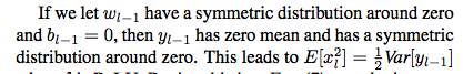
Hi! Does anybody else think that backward derivation in kaiming paper is a bit awkward (wrong?) w.r.t. \Delta y having size k^2d and \hat{W} being c-by- k^2d ?

c - num of input channels
d - num of output channels (i.e. filters)
k - kernel size

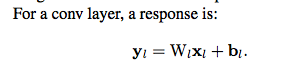
On forward pass you do: W @ x = (d, k^2*c) @ (k^2*c,) = (d,) - d channels of output pixel. For c=3, k=3 and d=10 we take 27 input pixels and produce 10 channels of output pixel. Makes sense.

On backward pass according to paper you do: W_hat @ delta(y) = (c, k^2*d) @ (k^2*d,) = (c,) - c gradients of input pixel. So with the example above for c=3, k=3 and d=10 we take 90(!) output gradients, multiply them by some 90 weights and produce only(!) 3 input gradients. Doesn’t make sense to me. Am I missing something?

In forward pass we got one pixel of d channels as output. So why then delta(y) is size k^2d and not just size d in backward? Shouldn’t backward pass be: transpose(W) @ delta(y) = (k^2*c, d) @ (d,) = (k^2*c,) to get back gradients of original k^2c input pixels? So for c=3, k=3 and d=10 we take 10 output gradients (one for each channel we output in forward pass) and produce 27 input gradients (one for each input pixel used).

I imagine that k^2d size of delta(y) somehow reflects the fact, that each of many (but not all!) input pixels is used in k^2 output pixels (for stride=1 convolution). So in backward phase each such pixel accumulates its gradient from k^2 output pixels, each piece being a sum of d products. That’s how (it seems to me) you get \hat{n} = k^2d.

But if previous statement is true, then Kaiming’s \hat{n} equals k^2d only for stride=1 convolutions where kernel size is non-significant compared to image size. Whereas for say k=3 stride=3 convolution \hat{n} = d instead of \hat{n} = k^2d because each input pixel is used only in 1 output pixel. Same for convolutions where image size is equal to kernel size, since each input pixel is again used only once. If kernel size is not too small compared to image size, \hat{n} will be something between d and k^2d.

Has anyone else bothered with this? I’ve read @PierreO blog post about inits, but there definition of \hat{n} is kinda skipped.